The linear algebra of deep learning

Strip away the terminology and a deep network is mostly matrix multiplication. Its layers multiply activations by weight matrices, its attention mechanism computes matrices of dot products, its convolutions are matrix products in disguise, and the cost of training and running it is counted in the floating-point operations of those products. This lesson applies the linear algebra of Lessons 1 and 2 to modern architectures: working with batched tensors and einsum notation, deriving scaled dot-product attention, writing convolution as a matrix, counting parameters and FLOPs, and using low-rank structure to fine-tune large models cheaply.

Tensors and batching

Deep learning frameworks work with tensors, arrays with any number of axes. A batch of token embeddings has shape (batch, sequence, width); a batch of images has shape (batch, channels, height, width). Matrix multiplication extends to tensors by treating leading axes as a batch: multiplying a (B, T, d) tensor by a (d, e) weight matrix applies the same linear map to every one of the B × T vectors, producing (B, T, e). This is why the same layer can process any batch size or sequence length.

Einstein summation (einsum) notation makes such operations explicit by naming every axis: an index that appears in the inputs but not in the output is summed over. "btd,de->bte" is the layer above; "bqd,bkd->bqk" computes every query–key dot product for every batch element; "bii->b" takes the trace of each matrix in a batch. Einsum is available in NumPy, PyTorch and JAX and is a reliable way to write, and read, tensor code without shape errors.

import numpy as np

rng = np.random.default_rng(15)
B, T, d = 2, 5, 8                        # batch, sequence length, model width
X = rng.normal(size=(B, T, d))
W = rng.normal(size=(d, 3 * d))

Y1 = X @ W                                # matmul broadcasts over the batch dimension
Y2 = np.einsum("btd,de->bte", X, W)       # the same, with every index named
print("Shapes:", X.shape, "@", W.shape, "->", Y1.shape, "| equal:", np.allclose(Y1, Y2))

Q, K = Y1[..., :d], Y1[..., d:2 * d]
S = np.einsum("bqd,bkd->bqk", Q, K)       # all query-key dot products, per batch
print("Attention score tensor:", S.shape)
print("Trace of each score matrix via einsum:", np.round(np.einsum("bii->b", S), 3))

Shapes: (2, 5, 8) @ (8, 24) -> (2, 5, 24) | equal: True
Attention score tensor: (2, 5, 5)
Trace of each score matrix via einsum: [ 10.356 115.878]

Layers are matrices

A fully connected layer computes \(\mathbf{h} = \phi(\mathbf{W}\mathbf{x} + \mathbf{b})\): a linear map followed by an elementwise nonlinearity \(\phi\) such as ReLU or GELU. Without the nonlinearity, stacking layers would be pointless, because a product of matrices is just another matrix. With it, each layer can bend and fold space, and composition builds complex functions. The linear-algebra view explains several practical facts:

• The rank of a layer's weight matrix bounds how many independent directions of information pass through it; a narrow layer is a bottleneck.
• The singular values of weight matrices control how much signals and gradients grow or shrink through each layer. If they are consistently above 1, activations and gradients explode with depth; below 1, they vanish. Initialization schemes (such as Xavier/Glorot and He initialization) choose weight variances so that singular values are near 1 at the start, and normalization layers and residual connections keep them well behaved during training.

Attention as matrix products

The transformer's attention mechanism computes, for each position, a weighted average of value vectors, with weights from the similarity between that position's query and every key. With queries \(\mathbf{Q}\), keys \(\mathbf{K}\) and values \(\mathbf{V}\) as matrices with one row per position, all positions are handled at once:

The \(T \times T\) matrix \(\mathbf{Q}\mathbf{K}^{T}\) holds every query–key dot product; softmax turns each row into weights that sum to 1 (computed stably as in Lesson 5); multiplying by \(\mathbf{V}\) forms the weighted averages. In a language model, a causal mask sets scores for future positions to \(-\infty\) so that each token attends only to earlier ones.

import numpy as np

def attention(Q, K, V, causal=True):
    d = Q.shape[-1]
    S = Q @ K.swapaxes(-1, -2) / np.sqrt(d)            # scaled scores
    if causal:                                          # each position sees only the past
        T = S.shape[-1]
        S = np.where(np.tril(np.ones((T, T), bool)), S, -np.inf)
    S = S - S.max(axis=-1, keepdims=True)               # stable softmax
    A = np.exp(S)
    A /= A.sum(axis=-1, keepdims=True)
    return A @ V, A

rng = np.random.default_rng(16)
T, d = 4, 64
Q, K, V = (rng.normal(size=(T, d)) for _ in range(3))
out, A = attention(Q, K, V)
print("Output shape:", out.shape, "| rows of A sum to 1:", np.allclose(A.sum(axis=1), 1))
print("Attention weights (causal):")
print(np.round(A, 3))
raw = Q @ K.T
print(f"Std of raw scores {raw.std():.2f} (about sqrt(d) = {np.sqrt(d):.1f}); after scaling {(raw / np.sqrt(d)).std():.2f}")

Output shape: (4, 64) | rows of A sum to 1: True
Attention weights (causal):
[[1.    0.    0.    0.   ]
 [0.495 0.505 0.    0.   ]
 [0.308 0.425 0.267 0.   ]
 [0.097 0.138 0.208 0.557]]
Std of raw scores 7.34 (about sqrt(d) = 8.0); after scaling 0.92

Why divide by \(\sqrt{d_{k}}\)? If query and key components are independent with unit variance, their dot product is a sum of \(d_{k}\) terms with variance \(d_{k}\), so its standard deviation is \(\sqrt{d_{k}}\) (Lesson 3). Unscaled scores of size 8 or more would make the softmax nearly one-hot, with tiny gradients for every other position; scaling restores unit variance.

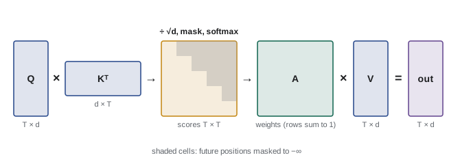
The \(T \times T\) score matrix is the cost of attention: its computation and memory grow with the square of the sequence length. For long contexts this dominates, which motivates memory-efficient implementations (such as FlashAttention, which computes the softmax in tiles without storing the whole matrix) and approximate attention methods.

Convolution as a matrix

A convolution slides a small filter across its input, computing a dot product at each position. Because it is linear, it can be written as multiplication by a matrix, one with a very special structure: each row is the same filter, shifted one place (a Toeplitz matrix in one dimension). The matrix is mostly zeros and shares the same few weights across all rows, which is exactly why convolutional layers have so few parameters and why they treat a feature the same wherever it appears.

import numpy as np

x = np.array([1.0, 2.0, 0.0, -1.0, 3.0, 1.0])
k = np.array([0.5, 1.0, -0.5])                       # a 3-tap filter
n_out = x.size - k.size + 1

T = np.zeros((n_out, x.size))                        # build the Toeplitz matrix
for i in range(n_out):
    T[i, i:i + k.size] = k[::-1]                     # flipped kernel: true convolution
print("Toeplitz matrix:")
print(T)
print("T @ x:          ", T @ x)
print("np.convolve:    ", np.convolve(x, k, mode="valid"))

Toeplitz matrix:
[[-0.5  1.   0.5  0.   0.   0. ]
 [ 0.  -0.5  1.   0.5  0.   0. ]
 [ 0.   0.  -0.5  1.   0.5  0. ]
 [ 0.   0.   0.  -0.5  1.   0.5]]
T @ x:           [ 1.5 -1.5  0.5  4. ]
np.convolve:     [ 1.5 -1.5  0.5  4. ]

Libraries sometimes implement 2-D convolutions literally this way, unrolling image patches into the columns of a matrix (im2col) so that the whole convolution becomes one large matrix multiplication on fast matrix hardware. Deep learning "convolution" layers usually compute cross-correlation (without flipping the filter); since the filter is learned, the distinction does not matter.

Counting parameters and FLOPs

Multiplying an \(m \times n\) matrix by an \(n \times p\) matrix takes \(mnp\) multiply-adds, or \(2mnp\) floating-point operations (FLOPs). Applied to a model, this gives quick, useful estimates. A standard transformer layer of width \(d\) has about \(4d^{2}\) attention parameters (query, key, value and output projections) and \(8d^{2}\) MLP parameters (with a hidden width of \(4d\)): about \(12d^{2}\) per layer. A forward pass costs about 2 FLOPs per parameter per token, plus the attention scores, and training (forward and backward) about 6 FLOPs per parameter per token: the "6ND" rule for \(N\) parameters and \(D\) training tokens.

d, layers, vocab, ctx = 4096, 32, 50_000, 4096
ffn = 4 * d

attn_params = 4 * d * d                       # Q, K, V and output projections
mlp_params = 2 * d * ffn                      # up and down projections
per_layer = attn_params + mlp_params
total = layers * per_layer + vocab * d        # plus the token embedding
print(f"Per layer: attention {attn_params / 1e6:.1f} M, MLP {mlp_params / 1e6:.1f} M, total {per_layer / 1e6:.1f} M")
print(f"Model: {total / 1e9:.2f} billion parameters")

flops_per_token = 2 * layers * per_layer + 2 * layers * ctx * d   # matmuls + attention scores
print(f"Forward pass: about {flops_per_token / 1e9:.1f} GFLOP per token")
tokens = 2e12
print(f"Training on {tokens:.0e} tokens: about {6 * total * tokens:.2e} FLOP (6 N D rule)")

Per layer: attention 67.1 M, MLP 134.2 M, total 201.3 M
Model: 6.65 billion parameters
Forward pass: about 14.0 GFLOP per token
Training on 2e+12 tokens: about 7.98e+22 FLOP (6 N D rule)

Low-rank structure and efficient fine-tuning

Fine-tuning a large model updates every weight matrix, requiring memory for gradients and optimizer states of every parameter. Low-rank adaptation (LoRA) instead freezes the pretrained weight \(\mathbf{W}\) and learns a low-rank correction:

The update has rank at most \(r\) and only \(r(d_{out} + d_{in})\) trainable parameters. It works because the weight changes needed to adapt a model to a new task turn out to be approximately low rank, so a truncated SVD (Lesson 1) of the change captures nearly all of it.

import numpy as np

rng = np.random.default_rng(17)
d_out, d_in, r = 1024, 1024, 8
full = d_out * d_in
lora = r * (d_out + d_in)
print(f"Full update: {full:,} parameters | LoRA rank {r}: {lora:,} ({100 * lora / full:.2f}%)")

# A weight change that is approximately low rank, plus small noise
delta = rng.normal(size=(d_out, r)) @ rng.normal(size=(r, d_in)) / np.sqrt(r) + 0.05 * rng.normal(size=(d_out, d_in))
U, s, Vt = np.linalg.svd(delta, full_matrices=False)
for k in [2, 8, 32]:
    approx = (U[:, :k] * s[:k]) @ Vt[:k]
    rel = np.linalg.norm(delta - approx) / np.linalg.norm(delta)
    print(f"rank {k:>2} approximation: relative error {rel:.3f}")

Full update: 1,048,576 parameters | LoRA rank 8: 16,384 (1.56%)
rank  2 approximation: relative error 0.843
rank  8 approximation: relative error 0.050
rank 32 approximation: relative error 0.047

A rank-8 update trains 1.6% of the layer's parameters, and when the true change is close to rank 8, a rank-8 approximation captures it almost completely: raising the rank to 32 adds little, because what remains is noise. The same low-rank idea appears in model compression, in grouped-query attention (sharing keys and values across heads) and in the analysis of what networks learn.