The multivariate Gaussian and Gaussian processes

Lesson 6 introduced random variables, covariance and the univariate Gaussian. In machine learning, almost everything is a vector, and the multivariate Gaussian is the distribution that ties linear algebra and probability together. It is the noise model behind least squares, the prior behind weight decay, the latent space of variational autoencoders and diffusion models, and the basis of Gaussian processes, a flexible way to learn functions with honest uncertainty. This lesson develops the multivariate Gaussian: its density and geometry, the Mahalanobis distance, sampling, the remarkable fact that its marginals and conditionals are also Gaussian, Bayesian linear regression, and Gaussian process regression.

The density and its geometry

A random vector \(\mathbf{x} \in \mathbb{R}^{d}\) has a multivariate Gaussian (normal) distribution with mean \(\boldsymbol{\mu}\) and covariance matrix \(\boldsymbol{\Sigma}\) if its density is

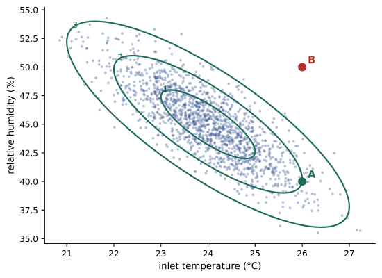
The covariance matrix is symmetric and positive definite. Its eigenvectors (Lesson 1) give the principal axes of the elliptical contours of constant density, and the square roots of its eigenvalues give the spread along each axis. A diagonal \(\boldsymbol{\Sigma}\) means independent components with axis-aligned ellipses; off-diagonal entries tilt the ellipses and express correlation.

The Mahalanobis distance

The quantity in the exponent defines the Mahalanobis distance \(D_{M}(\mathbf{x}) = \sqrt{(\mathbf{x} - \boldsymbol{\mu})^{T}\boldsymbol{\Sigma}^{-1}(\mathbf{x} - \boldsymbol{\mu})}\): the distance from the mean measured in standard deviations, taking correlations into account. Points on the same density contour have the same Mahalanobis distance. For anomaly detection it is far better than Euclidean distance, because it knows which combinations of values are normal.

import numpy as np

mu = np.array([24.0, 45.0])                        # inlet temperature (C), relative humidity (%)
Sigma = np.array([[1.0, -2.4],
                  [-2.4, 9.0]])                    # temperature and humidity move oppositely
L = np.linalg.cholesky(Sigma)                      # Sigma = L L^T
rng = np.random.default_rng(8)
samples = mu + rng.normal(size=(20_000, 2)) @ L.T
print("Sample mean:", np.round(samples.mean(axis=0), 2))
print("Sample covariance:", np.round(np.cov(samples.T), 2).tolist())

Sinv = np.linalg.inv(Sigma)
for name, p in [("A", np.array([26.0, 40.0])), ("B", np.array([26.0, 50.0]))]:
    d = p - mu
    print(f"Reading {name} {p}: Euclidean {np.linalg.norm(d):.2f}, Mahalanobis {np.sqrt(d @ Sinv @ d):.2f}")

Sample mean: [23.99 45.06]
Sample covariance: [[0.99, -2.39], [-2.39, 8.98]]
Reading A [26. 40.]: Euclidean 5.39, Mahalanobis 2.00
Reading B [26. 50.]: Euclidean 5.39, Mahalanobis 5.80

Readings A and B are equally far from the mean in Euclidean terms. But A (warmer and drier) follows the normal pattern, in which temperature and humidity move in opposite directions, and is only 2 standard deviations out; B (warmer and more humid) breaks the pattern and is 5.8 standard deviations out, a strong anomaly. For a \(d\)-dimensional Gaussian, \(D_{M}^{2}\) follows a chi-squared distribution with \(d\) degrees of freedom, which turns the distance into a principled alarm threshold.

Sampling and linear transformations

If \(\mathbf{z}\) is a vector of independent standard normals and \(\mathbf{x} = \boldsymbol{\mu} + \mathbf{A}\mathbf{z}\), then \(\mathbf{x}\) is Gaussian with mean \(\boldsymbol{\mu}\) and covariance \(\mathbf{A}\mathbf{A}^{T}\). More generally, any linear transformation of a Gaussian is Gaussian: \(\mathbf{y} = \mathbf{B}\mathbf{x} + \mathbf{b}\) has mean \(\mathbf{B}\boldsymbol{\mu} + \mathbf{b}\) and covariance \(\mathbf{B}\boldsymbol{\Sigma}\mathbf{B}^{T}\). To sample from a given \(\boldsymbol{\Sigma}\), factor it as \(\boldsymbol{\Sigma} = \mathbf{L}\mathbf{L}^{T}\) with the Cholesky decomposition (\(\mathbf{L}\) lower triangular) and set \(\mathbf{x} = \boldsymbol{\mu} + \mathbf{L}\mathbf{z}\), as the code above does.

The same idea, writing a random variable as a deterministic function of its parameters and independent noise, is the reparameterization trick that lets variational autoencoders and diffusion models backpropagate through sampling: \(\mathbf{x} = \boldsymbol{\mu}_{\theta} + \boldsymbol{\sigma}_{\theta} \odot \mathbf{z}\) is differentiable in \(\theta\) (Lesson 5).

Marginals and conditionals

Partition a Gaussian vector into two parts \(\mathbf{x} = (\mathbf{x}_{a}, \mathbf{x}_{b})\) with mean \((\boldsymbol{\mu}_{a}, \boldsymbol{\mu}_{b})\) and covariance blocks \(\boldsymbol{\Sigma}_{aa}, \boldsymbol{\Sigma}_{ab}, \boldsymbol{\Sigma}_{bb}\). Then:

• The marginal of \(\mathbf{x}_{a}\) is Gaussian with mean \(\boldsymbol{\mu}_{a}\) and covariance \(\boldsymbol{\Sigma}_{aa}\): simply drop the other variables.
• The conditional of \(\mathbf{x}_{b}\) given \(\mathbf{x}_{a}\) is Gaussian with

The conditional mean is a linear function of the observed values (it is exactly linear regression), and the conditional covariance is smaller than the marginal one and does not depend on the values observed. These two formulas are the engine of Kalman filters, Gaussian processes and Bayesian linear regression.

import numpy as np

mu = np.array([24.0, 45.0])
Sigma = np.array([[1.0, -2.4], [-2.4, 9.0]])
x0 = 26.0                                           # observed temperature
cond_mean = mu[1] + Sigma[1, 0] / Sigma[0, 0] * (x0 - mu[0])
cond_var = Sigma[1, 1] - Sigma[1, 0] ** 2 / Sigma[0, 0]
print(f"Humidity given temperature 26 C: mean {cond_mean:.2f} %, std {np.sqrt(cond_var):.2f} % "
      f"(unconditional std {np.sqrt(Sigma[1, 1]):.2f} %)")

rng = np.random.default_rng(9)
s = mu + rng.normal(size=(400_000, 2)) @ np.linalg.cholesky(Sigma).T
near = s[np.abs(s[:, 0] - x0) < 0.05, 1]           # samples with temperature close to 26 C
print(f"Monte Carlo check from {near.size} samples: mean {near.mean():.2f} %, std {near.std():.2f} %")

Humidity given temperature 26 C: mean 40.20 %, std 1.80 % (unconditional std 3.00 %)
Monte Carlo check from 2175 samples: mean 40.14 %, std 1.80 %

Observing a temperature of 26 °C (2 standard deviations above its mean) shifts the expected humidity down from 45% to 40.2%, because of the negative correlation, and shrinks its standard deviation from 3.0% to 1.8%: knowing one correlated variable tells us something about the other.

Bayesian linear regression

Combine a Gaussian likelihood, \(\mathbf{y} \mid \mathbf{w} \sim \mathcal{N}(\mathbf{X}\mathbf{w}, \sigma^{2}\mathbf{I})\), with a Gaussian prior on the weights, \(\mathbf{w} \sim \mathcal{N}(\mathbf{0}, \tau^{2}\mathbf{I})\). Because everything is Gaussian, the posterior is Gaussian too, with

The posterior mean is exactly the ridge regression solution with \(\lambda = \sigma^{2}/\tau^{2}\), the MAP estimate of Lesson 6, but the Bayesian treatment also gives the posterior covariance, which quantifies uncertainty in the weights and therefore in every prediction.

import numpy as np

rng = np.random.default_rng(10)
true_w = np.array([1.0, 0.5])
noise_sd, prior_sd = 0.5, 2.0

def posterior(X, y):
    A = X.T @ X / noise_sd**2 + np.eye(2) / prior_sd**2       # posterior precision
    cov = np.linalg.inv(A)
    mean = cov @ X.T @ y / noise_sd**2
    return mean, cov

x_new = np.array([1.0, 8.0])                                   # predict at x = 8
for n in [2, 10, 100]:
    x = rng.uniform(0, 5, n)
    X = np.column_stack([np.ones(n), x])
    y = X @ true_w + rng.normal(0, noise_sd, n)
    m, C = posterior(X, y)
    pred_sd = np.sqrt(x_new @ C @ x_new + noise_sd**2)
    print(f"n = {n:>3}: posterior mean {np.round(m, 3)}, weight sds {np.round(np.sqrt(np.diag(C)), 3)}, "
          f"prediction at x = 8: {x_new @ m:.2f} +/- {2 * pred_sd:.2f}")

n =   2: posterior mean [1.165 0.387], weight sds [0.62  0.182], prediction at x = 8: 4.26 +/- 2.24
n =  10: posterior mean [0.405 0.603], weight sds [0.415 0.127], prediction at x = 8: 5.23 +/- 1.65
n = 100: posterior mean [0.782 0.522], weight sds [0.104 0.039], prediction at x = 8: 4.96 +/- 1.10

The predictive interval combines uncertainty about the weights with the noise in the observations; as data accumulates, the weight uncertainty shrinks toward zero but the noise remains, so the interval approaches about ±2σ = ±1.0. Note also that x = 8 lies beyond the training range (0 to 5): a model that reports its uncertainty warns when it is extrapolating.

Gaussian processes

A Gaussian process (GP) extends the multivariate Gaussian to functions: it is a distribution over functions \(f\) such that the values at any finite set of inputs are jointly Gaussian, with covariances given by a kernel (Lesson 3), \(\text{Cov}(f(x), f(x^{\prime})) = k(x, x^{\prime})\). The RBF kernel encodes the belief that nearby inputs have similar outputs. Given noisy observations at training inputs, predictions at new inputs follow directly from the Gaussian conditioning formula:

import numpy as np

def rbf(a, b, length=1.0, var=1.0):
    return var * np.exp(-0.5 * (a[:, None] - b[None, :]) ** 2 / length**2)

x_train = np.array([0.5, 1.5, 2.0, 4.0, 5.5, 6.0])
y_train = np.sin(x_train)
noise = 1e-4
x_test = np.array([1.0, 3.0, 5.0, 8.0])

K = rbf(x_train, x_train) + noise * np.eye(x_train.size)
Ks = rbf(x_test, x_train)
mean = Ks @ np.linalg.solve(K, y_train)
cov = rbf(x_test, x_test) - Ks @ np.linalg.solve(K, Ks.T)
sd = np.sqrt(np.clip(np.diag(cov), 0, None))
for x, m, s in zip(x_test, mean, sd):
    print(f"x = {x:.1f}: prediction {m:+.3f} +/- {2 * s:.3f}   (true sin x = {np.sin(x):+.3f})")

x = 1.0: prediction +0.807 +/- 0.189   (true sin x = +0.841)
x = 3.0: prediction +0.082 +/- 0.797   (true sin x = +0.141)
x = 5.0: prediction -0.979 +/- 0.366   (true sin x = -0.959)
x = 8.0: prediction +0.095 +/- 1.952   (true sin x = +0.989)

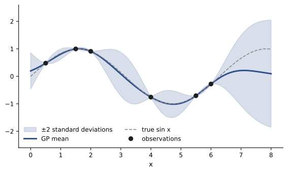
At x = 1 and x = 5, close to data, the predictions are accurate and the intervals narrow. At x = 3, in a gap, the interval widens. At x = 8, far beyond the data, the mean falls back to the prior mean of zero and the interval spans almost the whole prior range: the model correctly says it does not know. This honest uncertainty makes GPs the method of choice for Bayesian optimization, which tunes expensive experiments and hyperparameters (AI-310), and for problems with little data. Their cost, an \(n \times n\) solve, limits exact GPs to some thousands of points, though sparse approximations extend them further.