
AI-210 · Lesson 4 of 12 · 34 min
Matrix calculus and gradients
Training a machine learning model means adjusting its parameters to reduce a loss function, and the tool for doing that is the gradient: the vector of partial derivatives that points in the direction of steepest increase. A modern neural network has millions or billions of parameters, and every training step computes the gradient of the loss with respect to all of them. The method that makes this feasible, backpropagation, is nothing more than the chain rule of calculus organized efficiently, and it is what deep learning frameworks such as PyTorch and JAX automate.
This chapter builds the calculus needed to understand it: gradients, directional derivatives, Jacobians and Hessians; the handful of matrix derivative identities used constantly; the least-squares solution derived by setting a gradient to zero; the gradient of the softmax cross-entropy loss; and backpropagation through a small network, checked numerically.
Gradients and directional derivatives
For a scalar function of a vector, \(f: \mathbb{R}^n \to \mathbb{R}\), the gradient collects the partial derivatives:
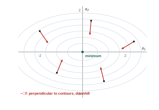
The rate of change of \(f\) in the direction of a unit vector \(\mathbf{u}\) is the directional derivative \(\nabla f^\top\mathbf{u} = \|\nabla f\|\cos\theta\). It is largest when \(\mathbf{u}\) points along the gradient, so the gradient is the direction of steepest ascent and \(-\nabla f\) the direction of steepest descent; its length is the steepest slope. Gradient descent, \(\mathbf{x} \leftarrow \mathbf{x} - \eta\nabla f(\mathbf{x})\), takes small steps downhill. The gradient is also perpendicular to the contour lines (level sets) of \(f\).
Worked problem
Gradient and directional derivative
For \(f(x_1, x_2) = x_1^2 + 3x_1x_2 + 2x_2^2\), find \(\nabla f\) at (1, 2), the steepest slope there, and the directional derivative along \(\mathbf{u} = (0.8, -0.6)\).
Show solution
- \(\partial f/\partial x_1 = 2x_1 + 3x_2 = 2 + 6 = 8\); \(\partial f/\partial x_2 = 3x_1 + 4x_2 = 3 + 8 = 11\). So \(\nabla f = (8, 11)\).
- Steepest slope: \(\|\nabla f\| = \sqrt{64 + 121} = 13.6\).
- Along \(\mathbf{u}\): \(8 \times 0.8 + 11 \times (-0.6) = 6.4 - 6.6 = -0.2\).
Answer: \(\nabla f = (8, 11)\), steepest slope 13.6, and −0.2 along \(\mathbf{u}\): that direction is almost along a contour line, so \(f\) barely changes.
Jacobians and Hessians
For a vector-valued function \(\mathbf{f}: \mathbb{R}^n \to \mathbb{R}^m\), the derivative is the \(m \times n\) Jacobian matrix \(\mathbf{J}\), with \(J_{ij} = \partial f_i/\partial x_j\). It is the best linear approximation of \(\mathbf{f}\) near a point: \(\mathbf{f}(\mathbf{x} + \boldsymbol{\delta}) \approx \mathbf{f}(\mathbf{x}) + \mathbf{J}\boldsymbol{\delta}\). Two cases appear constantly in neural networks:
- A linear layer \(\mathbf{f}(\mathbf{x}) = \mathbf{A}\mathbf{x}\) has Jacobian \(\mathbf{J} = \mathbf{A}\).
- An element-wise function such as \(\tanh\) or ReLU has a diagonal Jacobian, \(\operatorname{diag}(\sigma\prime(x_1), \dots, \sigma\prime(x_n))\), because each output depends only on its own input. In code it is never formed as a matrix; it is simply an element-wise multiplication.
The second derivatives of a scalar function form the Hessian, \(H_{ij} = \partial^2 f/\partial x_i\,\partial x_j\), a symmetric \(n \times n\) matrix describing curvature. It gives the quadratic approximation \(f(\mathbf{x} + \boldsymbol{\delta}) \approx f(\mathbf{x}) + \nabla f^\top\boldsymbol{\delta} + \tfrac12\boldsymbol{\delta}^\top\mathbf{H}\boldsymbol{\delta}\). At a point where the gradient is zero, a positive definite Hessian means a local minimum, a negative definite one a local maximum, and an indefinite one (eigenvalues of both signs) a saddle point.
Worked problem
Classifying a stationary point
For \(f = x_1^2 + 3x_1x_2 + 2x_2^2\), find the Hessian and decide what kind of point the origin is.
Show solution
- \(\mathbf{H} = \begin{bmatrix} 2 & 3 \ 3 & 4 \end{bmatrix}\), the same everywhere because \(f\) is quadratic.
- At the origin \(\nabla f = 0\). \(\det\mathbf{H} = 8 - 9 = -1 < 0\), so the eigenvalues have opposite signs.
Answer: The origin is a saddle point: the function curves up in one direction and down in another. In high-dimensional neural network losses, saddle points are far more common than local minima, a point Lesson 11 returns to.
Identities for matrix derivatives
A small set of results, all derivable from the component definitions, covers most of what is needed. For vectors \(\mathbf{x}, \mathbf{a}\) and a matrix \(\mathbf{A}\):
| Function | Gradient with respect to x |
|---|---|
| \(\mathbf{a}^\top\mathbf{x}\) | \(\mathbf{a}\) |
| \(\mathbf{x}^\top\mathbf{x} = \|\mathbf{x}\|^2\) | \(2\mathbf{x}\) |
| \(\mathbf{x}^\top\mathbf{A}\mathbf{x}\) | \((\mathbf{A} + \mathbf{A}^\top)\mathbf{x}\), or \(2\mathbf{A}\mathbf{x}\) if \(\mathbf{A}\) is symmetric |
| \(\|\mathbf{A}\mathbf{x} - \mathbf{b}\|^2\) | \(2\mathbf{A}^\top(\mathbf{A}\mathbf{x} - \mathbf{b})\) |
A useful habit is to check shapes: the gradient of a scalar with respect to \(\mathbf{x} \in \mathbb{R}^n\) must itself be in \(\mathbb{R}^n\), so for example \(\mathbf{A}^\top(\mathbf{A}\mathbf{x} - \mathbf{b})\) has the right shape (\(n \times m\) times \(m\)), while \(\mathbf{A}(\mathbf{A}\mathbf{x} - \mathbf{b})\) would not even be defined for a non-square \(\mathbf{A}\).
Least squares from the gradient
Linear regression fits weights \(\mathbf{w}\) to minimize the squared error \(L(\mathbf{w}) = \|\mathbf{X}\mathbf{w} - \mathbf{y}\|^2\) over \(N\) examples. By the last identity, \(\nabla L = 2\mathbf{X}^\top(\mathbf{X}\mathbf{w} - \mathbf{y})\). Setting it to zero gives the normal equations and their solution:
Because \(L\) is a convex quadratic (its Hessian \(2\mathbf{X}^\top\mathbf{X}\) is positive semidefinite), this stationary point is the global minimum. In practice the system is solved with a factorization rather than an explicit inverse.
Worked problem
A one-parameter fit
Fit \(y = wx\) (no intercept) to the points (1, 2), (2, 3), (3, 5).
Show solution
- With one feature, the normal equation is \(w\sum x_i^2 = \sum x_iy_i\).
- \(\sum x_i^2 = 1 + 4 + 9 = 14\); \(\sum x_iy_i = 2 + 6 + 15 = 23\).
- \(w = 23/14 = 1.643\).
Answer: \(w \approx 1.64\). The same formula, in matrix form, fits models with thousands of features.
The program below checks the least-squares gradient numerically and then solves the normal equations. Checking an analytic gradient against finite differences is the standard way to catch derivation and coding errors.
import numpy as np

rng = np.random.default_rng(0)
X = rng.normal(size=(50, 3))
y = X @ np.array([1.5, -2.0, 0.5]) + 0.1 * rng.normal(size=50)
w = np.zeros(3)

def loss(w):
    r = X @ w - y
    return r @ r                      # sum of squared residuals

grad = 2 * X.T @ (X @ w - y)          # analytic gradient

eps = 1e-6                            # central differences, one coordinate at a time
num = np.array([(loss(w + eps * e) - loss(w - eps * e)) / (2 * eps) for e in np.eye(3)])
print("analytic :", grad.round(4))
print("numerical:", num.round(4))
print("agree:", np.allclose(grad, num, rtol=1e-6))
w_star = np.linalg.solve(X.T @ X, X.T @ y)       # set the gradient to zero
print("least-squares weights:", w_star.round(3))analytic : [-182.2827 129.706 -60.6253] numerical: [-182.2827 129.706 -60.6253] agree: True least-squares weights: [ 1.518 -2.016 0.502]
The recovered weights (1.518, −2.016, 0.502) are close to the true (1.5, −2.0, 0.5) used to generate the data; the small differences come from the noise.
The chain rule
Most functions in machine learning are compositions: a loss of a prediction of a layer of a layer. The chain rule handles them. For scalars, if \(y = f(u)\) and \(u = g(x)\), then \(dy/dx = (dy/du)(du/dx)\). For vectors, Jacobians multiply: if \(\mathbf{y} = \mathbf{f}(\mathbf{u})\) and \(\mathbf{u} = \mathbf{g}(\mathbf{x})\), then \(\mathbf{J}_{\mathbf{y}\mathbf{x}} = \mathbf{J}_{\mathbf{y}\mathbf{u}}\mathbf{J}_{\mathbf{u}\mathbf{x}}\).
Worked problem
The gradient of a single neuron
A neuron computes \(z = wx + b\), \(\hat{y} = \sigma(z)\) with the logistic sigmoid \(\sigma(z) = 1/(1 + e^{-z})\), and loss \(L = \tfrac12(\hat{y} - t)^2\). With \(w = 2\), \(x = 1\), \(b = -1\) and target \(t = 1\), find \(\partial L/\partial w\).
Show solution
- Forward: \(z = 2 - 1 = 1\); \(\hat{y} = \sigma(1) = 0.731\); \(L = \tfrac12(0.731 - 1)^2 = 0.036\).
- \(\partial L/\partial\hat{y} = \hat{y} - t = -0.269\).
- \(\partial\hat{y}/\partial z = \sigma(z)(1 - \sigma(z)) = 0.731 \times 0.269 = 0.197\).
- \(\partial z/\partial w = x = 1\).
- \(\partial L/\partial w = -0.269 \times 0.197 \times 1 = -0.0529\).
Answer: \(\partial L/\partial w = -0.053\). The negative sign says increasing \(w\) reduces the loss, so gradient descent will increase it, pushing the prediction toward the target.
Softmax and cross-entropy
Classifiers with \(K\) classes output \(K\) scores (logits) \(\mathbf{z}\), turned into probabilities by the softmax function, and are trained with the cross-entropy loss against a one-hot target \(\mathbf{y}\) (Lesson 9 explains why):
Working through the derivatives, the softmax and the logarithm combine into a remarkably simple gradient:
The gradient is just the predicted probabilities minus the target: it pushes up the logit of the correct class by how far its probability falls short of 1, and pushes down every other logit by its probability. This clean result is one reason softmax and cross-entropy are always used together.
import numpy as np

def softmax(z):
    e = np.exp(z - z.max())           # subtract the max for numerical stability
    return e / e.sum()

z = np.array([2.0, 1.0, 0.1])         # logits for 3 classes
y = np.array([0.0, 1.0, 0.0])         # true class is class 1
p = softmax(z)
L = -np.sum(y * np.log(p))
print("p =", p.round(4), " loss =", round(L, 4))
print("gradient p - y =", (p - y).round(4))

eps = 1e-6
num = np.array([(-np.sum(y * np.log(softmax(z + eps * e))) - -np.sum(y * np.log(softmax(z - eps * e)))) / (2 * eps)
                for e in np.eye(3)])
print("numerical =", num.round(4))p = [0.659 0.2424 0.0986] loss = 1.417 gradient p - y = [ 0.659 -0.7576 0.0986] numerical = [ 0.659 -0.7576 0.0986]
Subtracting the maximum logit before exponentiating does not change the softmax (it cancels in the ratio) but prevents overflow when logits are large, a standard numerical precaution.
Backpropagation
Lesson 5 shows how frameworks automate what follows for any program, and the numerical precision it runs in.
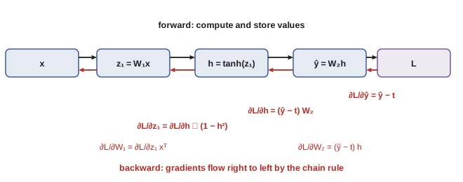
A neural network is a chain of layers, and its loss is a composition of many functions. Backpropagation computes the gradient of the loss with respect to every parameter by applying the chain rule from the output backwards. A forward pass computes and stores each layer's output. A backward pass then starts with \(\partial L/\partial\hat{y}\) and, layer by layer, multiplies by each layer's local derivative, producing at each layer both the gradient for that layer's parameters and the gradient to pass to the layer below.
import numpy as np

rng = np.random.default_rng(42)
x = rng.normal(size=4)                 # one input
t = 1.0                                # target
W1 = rng.normal(size=(3, 4)); W2 = rng.normal(size=3)

def forward(W1, W2):
    h = np.tanh(W1 @ x)                # hidden layer
    yhat = W2 @ h                      # output
    return 0.5 * (yhat - t) ** 2, h, yhat

L, h, yhat = forward(W1, W2)
# Backpropagation: apply the chain rule from the loss backwards
dy = yhat - t                          # dL/dyhat
dW2 = dy * h                           # dL/dW2
dh = dy * W2                           # dL/dh
dz = dh * (1 - h ** 2)                 # through tanh: d tanh(z)/dz = 1 - tanh^2
dW1 = np.outer(dz, x)                  # dL/dW1

eps = 1e-6
E = np.zeros_like(W1); E[1, 2] = eps   # check one entry of dW1
num = (forward(W1 + E, W2)[0] - forward(W1 - E, W2)[0]) / (2 * eps)
print(f"loss {L:.4f}")
print(f"backprop dL/dW1[1,2] = {dW1[1, 2]:.6f}")
print(f"numerical = {num:.6f}")loss 3.2841 backprop dL/dW1[1,2] = 0.076549 numerical = 0.076549
Notice the pattern: the gradient for a weight matrix is always an outer product of the gradient arriving from above and the input that the layer received in the forward pass. That is why training needs memory to store activations, which in large models is often a bigger constraint than storing the weights themselves.
Why reverse mode
There are two ways to apply the chain rule through a long composition. Forward mode carries derivatives along with values from input to output, which costs one pass per input variable. Reverse mode, backpropagation, carries them from output to input, which costs one backward pass per output. A training loss has millions of inputs (parameters) and one output (the loss), so reverse mode computes the full gradient in roughly the time of two or three forward passes, while forward mode would need millions. Automatic differentiation libraries implement reverse mode generally: they record the operations of the forward pass and replay them backwards, so practitioners rarely write gradients by hand. Understanding what they compute, and checking gradients numerically when writing custom operations, remains essential.
Common mistakes
MistakeForgetting the transpose in gradients such as \(2\mathbf{X}^\top(\mathbf{X}\mathbf{w} - \mathbf{y})\).
InsteadCheck shapes: the gradient must have the same shape as the variable.
MistakeUsing \(2\mathbf{A}\mathbf{x}\) as the gradient of \(\mathbf{x}^\top\mathbf{A}\mathbf{x}\) for a non-symmetric \(\mathbf{A}\).
InsteadThe general result is \((\mathbf{A} + \mathbf{A}^\top)\mathbf{x}\).
MistakeChecking gradients with one-sided differences and a tiny step.
InsteadUse central differences, \((f(x + \epsilon) - f(x - \epsilon))/2\epsilon\), with \(\epsilon \approx 10^{-6}\) in double precision.
MistakeComputing softmax as exp(z)/sum(exp(z)) directly.
InsteadSubtract the maximum logit first to avoid overflow.
MistakeAssuming a zero gradient means a minimum.
InsteadCheck the Hessian: it may be a maximum or a saddle point.
Summary and key terms
- The gradient \(\nabla f\) points uphill; its length is the steepest slope; the directional derivative is \(\nabla f^\top\mathbf{u}\).
- Jacobians are matrices of first derivatives of vector functions; Hessians are symmetric matrices of second derivatives.
- Key identities: \(\nabla(\mathbf{a}^\top\mathbf{x}) = \mathbf{a}\), \(\nabla(\mathbf{x}^\top\mathbf{A}\mathbf{x}) = (\mathbf{A} + \mathbf{A}^\top)\mathbf{x}\), \(\nabla\|\mathbf{A}\mathbf{x} - \mathbf{b}\|^2 = 2\mathbf{A}^\top(\mathbf{A}\mathbf{x} - \mathbf{b})\).
- Setting the least-squares gradient to zero gives the normal equations \(\mathbf{X}^\top\mathbf{X}\mathbf{w} = \mathbf{X}^\top\mathbf{y}\).
- At a stationary point, a positive definite Hessian means a minimum and an indefinite one a saddle.
- The chain rule multiplies local derivatives (Jacobians) along a composition.
- Softmax with cross-entropy has the gradient \(\mathbf{p} - \mathbf{y}\).
- Backpropagation is reverse-mode differentiation: one backward pass gives the gradient for all parameters; verify custom gradients numerically.
- Gradient
- The vector of partial derivatives of a scalar function, pointing in the direction of steepest increase.
- Directional derivative
- The rate of change of a function along a given unit direction.
- Jacobian
- The matrix of first partial derivatives of a vector-valued function.
- Hessian
- The symmetric matrix of second partial derivatives of a scalar function.
- Stationary point
- A point where the gradient is zero.
- Saddle point
- A stationary point that is a minimum in some directions and a maximum in others.
- Normal equations
- The linear system \(\mathbf{X}^\top\mathbf{X}\mathbf{w} = \mathbf{X}^\top\mathbf{y}\) solved by least squares.
- Chain rule
- The rule for differentiating compositions by multiplying derivatives.
- Logits
- The unnormalized scores a classifier produces before the softmax.
- Softmax
- The function converting logits into probabilities that sum to one.
- Cross-entropy loss
- The negative log-probability the model assigns to the correct class.
- Backpropagation
- Computing gradients of a loss with respect to all parameters by applying the chain rule backwards.
- Automatic differentiation
- Software that computes exact derivatives of programs by recording and replaying operations.
- Gradient checking
- Comparing an analytic gradient with finite-difference estimates to detect errors.
Practice problems
Work each problem on paper first, then reveal the answer to check.
Find the gradient of \(f(x, y) = x^2y + \sin y\).
Show answer
∇f = (2xy, x² + cos y).
For \(f = 3x_1^2 + x_2^2\), find the gradient at (1, 2) and the steepest slope.
Show answer
∇f = (6, 4); slope √52 = 7.21.
What is the Jacobian of \(\mathbf{f}(\mathbf{x}) = (x_1x_2, x_1 + x_2)\)?
Show answer
[[x₂, x₁], [1, 1]].
Find the Hessian of \(f = x_1^2 + x_1x_2 + 3x_2^2\) and classify the origin.
Show answer
H = [[2, 1], [1, 6]]; det = 11 > 0 and trace > 0, so positive definite: a minimum.
Using the identities, find \(\nabla_{\mathbf{w}}\) of \(\|\mathbf{X}\mathbf{w} - \mathbf{y}\|^2 + \lambda\|\mathbf{w}\|^2\).
Show answer
2Xᵀ(Xw − y) + 2λw.
Setting the gradient from the previous question to zero, what is the solution (ridge regression)?
Show answer
w = (XᵀX + λI)⁻¹Xᵀy.
Fit \(y = wx\) to (1, 1), (2, 3), (4, 7).
Show answer
w = Σxy/Σx² = (1 + 6 + 28)/(1 + 4 + 16) = 35/21 = 1.667.
A softmax gives \(\mathbf{p} = (0.1, 0.7, 0.2)\) and the true class is 3. What is the gradient of the cross-entropy with respect to the logits?
Show answer
p − y = (0.1, 0.7, −0.8).
What is the derivative of ReLU, \(\max(0, z)\), and what is its Jacobian for a vector input?
Show answer
1 for z > 0 and 0 for z < 0 (undefined at 0, taken as 0 in practice); the Jacobian is diagonal with those values.
Why does training a network need to store the activations from the forward pass?
Show answer
Each weight gradient is an outer product of the backward gradient and the layer's forward input, and derivatives such as tanh′ need the forward values, so the backward pass reuses them.
Lesson quiz · 5 questions
Score 60% or more to complete this lesson.
Create a free account to save your progress, take quizzes and earn a certificate.