Pricing I: costs, value and elasticity

Lesson 1's value driver tree showed that a 1 percent change in price moves Northgate's ROCE more than any other lever. Yet pricing is often the least analyzed decision in a company. Prices are set by adding a markup to cost, by matching competitors, or by habit, and revisited only when something goes wrong. This lesson examines the three broad bases for pricing, which are cost, customers' perceived value and competition, and develops the economics of price and demand that underlie them. It applies them to setting the launch price for GrainSense, using results from regional price tests. Lesson 8 continues with target costing, life-cycle costing, pricing strategies and the legal limits on pricing.

Three bases for pricing

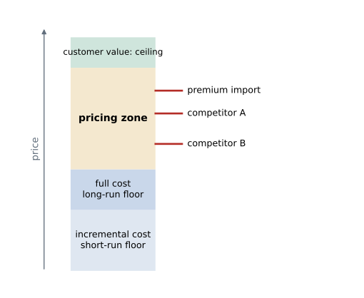
Every price decision balances three considerations. Costs set a floor in the long run: a business that cannot cover its full costs over time will not survive, and in the short run, a price below incremental cost loses money on every unit. Customers' perceived value sets a ceiling: no one will pay more than a product is worth to them compared with the alternatives. Competitors' prices shape where, between floor and ceiling, a price can be set. Good pricing decisions use information about all three. Problems arise when one is used to the exclusion of the others: cost-plus pricing that ignores value leaves money on the table or prices products out of the market; value pricing that ignores cost can sell profitable-looking volume at a loss; competitive pricing that ignores both can start price wars nobody wins.

Cost-plus pricing

Cost-plus pricing sets the price by adding a markup to a cost base. The base may be variable cost, full manufacturing cost or full cost including selling and administrative costs; the markup is chosen to cover any costs left out of the base and to provide a target profit. Cost-plus pricing is common because it is simple, easy to justify to customers and regulators, and, in industries where all firms use similar cost bases and markups, it tends to stabilize prices. It is widely used in contracting, where a cost-plus contract reimburses allowable costs plus a fee, and in regulated industries.

Its weaknesses are serious. It ignores demand: the same markup is applied whether customers would happily pay much more or will buy almost nothing at that price. It is circular: full cost per unit depends on volume, which depends on price. When volume falls, fixed costs are spread over fewer units, full cost per unit rises, the cost-plus price rises, and volume falls further. This is sometimes called the death spiral. And it can reward inefficiency, because higher costs lead to higher prices rather than to pressure to reduce them.

Value-based pricing

Value-based pricing starts from what the product is worth to customers. For business customers, that worth can often be estimated in money. The economic value to the customer is the price of the next best alternative plus the value of any additional benefits the product provides, less any additional costs it imposes. A farmer who loses grain to spoilage in storage loses its full market value; if GrainSense prevents, on average, the loss of a few hundred bushels a year, its value to that farmer can be estimated from crop prices, bin sizes and spoilage rates.

Northgate's product team estimates that for a typical farm with eight storage bins, GrainSense would avoid spoilage worth between 600 and 1,400 dollars a year, depending on the crop and the season, and might reduce insurance premiums for farmers whose insurers offer discounts for monitoring. Against this, a farmer could monitor bins manually with probes and regular checks, at a cost in time, or buy a competitor's simpler product priced at about 449 dollars. The analysis suggests that a price somewhere between 400 and 550 dollars per kit would leave most farmers better off, but it cannot say where within that range profit would be highest. For that, Northgate needs to know how demand responds to price.

Demand and price elasticity

A demand curve shows the quantity customers would buy at each price. The price elasticity of demand measures how responsive quantity is to price: it is the percentage change in quantity divided by the percentage change in price. Because demand curves slope downward, elasticity is negative; analysts often quote its absolute value. Demand is elastic when the absolute value exceeds one, so that a price increase reduces revenue, and inelastic when it is less than one, so that a price increase raises revenue.

Elasticity depends on the availability of substitutes, the share of the buyer's budget the product represents, how essential it is, and the time allowed for adjustment. Replacement parts for equipment that is already installed tend to have inelastic demand, which is why parts and service often earn higher margins than original equipment. New products competing with established alternatives tend to have more elastic demand.

Elasticity can be estimated in several ways: from historical sales and prices, if prices have varied enough and other influences can be controlled for; from surveys and conjoint analysis, which ask customers to choose between products with different features and prices; and from experiments, which offer different prices in comparable markets. Northgate used experiments. In the spring of 2026, it sold a pilot version of GrainSense through dealers in five comparable regions at five different prices, from 380 to 540 dollars, and scaled each region's sales to the size of the full market.

Finding the profit-maximizing price

With a linear demand curve, Q = a − bP, revenue is P × Q and profit is (P − v) × Q − F, where v is variable cost per unit and F is fixed cost. Profit is highest where marginal revenue equals marginal cost. For linear demand and constant variable cost, this gives a simple formula: the optimal price is halfway between the variable cost and the price at which demand falls to zero, a/b.

An equivalent result, valid for any demand curve, expresses the optimal price as a markup on marginal cost that depends only on elasticity: the more elastic the demand, the lower the markup.

Grace fits a demand line to the test results and compares three candidate prices: the sales team's cost-plus proposal, the profit-maximizing price and a low launch price intended to build share quickly.

# Pricing the GrainSense kit: estimate demand from regional price tests, then find the best price.
import random
random.seed(7)
test_prices = [380, 420, 460, 500, 540]
# simulated first-season unit sales in comparable test regions (scaled to the full market)
sales = [round(9800 - 13.0 * p + random.gauss(0, 180)) for p in test_prices]
print('Test results:', dict(zip(test_prices, sales)))
# least-squares line  Q = a - b P
n = len(test_prices); mp = sum(test_prices) / n; mq = sum(sales) / n
b = -sum((p - mp) * (q - mq) for p, q in zip(test_prices, sales)) / sum((p - mp) ** 2 for p in test_prices)
a = mq + b * mp
print(f"Estimated demand: Q = {a:,.0f} - {b:.2f} P")
vc, fixed = 190.0, 0.62e6          # variable cost per kit; annual fixed costs of the product line

def profit(p):
    q = max(a - b * p, 0)
    return q, (p - vc) * q - fixed

p_star = (a / b + vc) / 2          # where marginal revenue equals marginal cost
q_star, prof_star = profit(p_star)
elast = -b * p_star / q_star
full_cost = vc + fixed / 5000      # full cost per kit at a planned volume of 5,000
cost_plus = full_cost * 1.40       # the sales team's cost-plus proposal (40% markup)
for label, p in [('Cost-plus', cost_plus), ('Profit-maximizing', p_star), ('Low launch price', 380)]:
    q, pr = profit(p)
    print(f"{label:18s} price {p:6.0f}  units {q:6,.0f}  profit {pr:12,.0f}")
print(f"Price elasticity of demand at the optimum: {elast:.2f}")
print(f"Markup on variable cost at the optimum: {p_star / vc - 1:.0%}; "
      f"check rule p = VC x e/(1+e): {vc * elast / (1 + elast):.0f}")
# the cost-plus trap: recompute full cost at the volume the price actually sells
p, vol = cost_plus, 5000
for rnd in range(1, 4):
    vol = max(a - b * p, 1)
    p = (vc + fixed / vol) * 1.40
    print(f"Cost-plus round {rnd}: volume {vol:6,.0f} -> new full-cost price {p:6.0f}")

Test results: {380: 4814, 420: 4432, 460: 3779, 500: 3243, 540: 2613}
Estimated demand: Q = 10,206 - 13.98 P
Cost-plus          price    440  units  4,061  profit      393,711
Profit-maximizing  price    460  units  3,775  profit      399,574
Low launch price   price    380  units  4,894  profit      309,936
Price elasticity of demand at the optimum: -1.70
Markup on variable cost at the optimum: 142%; check rule p = VC x e/(1+e): 460
Cost-plus round 1: volume  4,061 -> new full-cost price    480
Cost-plus round 2: volume  3,501 -> new full-cost price    514
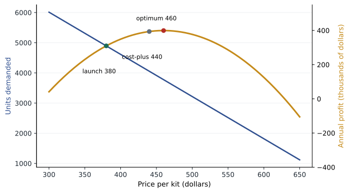
Cost-plus round 3: volume  3,022 -> new full-cost price    553

The estimated demand line is Q = 10,206 − 13.98P: each 1-dollar increase in price reduces annual sales by about 14 kits. With variable cost of 190 dollars and product-line fixed costs of 620,000 dollars a year, the profit-maximizing price is about 460 dollars, giving sales of about 3,775 kits and profit of about 400,000 dollars. Elasticity at that price is −1.70, and the markup rule confirms the price: 190 × 1.70 ÷ 0.70 = 460.

Three further points stand out. First, the sales team's cost-plus price of 440 dollars, based on full cost at a planned volume of 5,000 kits, is close to optimal and earns almost as much. The profit curve is flat near its peak, so modest errors in price cost little. Second, the cost-plus logic is unstable. At 440 dollars, Northgate would sell about 4,060 kits, not 5,000, so full cost per kit would be higher. Recalculating the cost-plus price at the volume actually sold gives 480 dollars, then 514, then 553, as volume falls each time: the death spiral in miniature. Third, the low launch price of 380 dollars sells nearly 5,000 kits but earns less, about 310,000 dollars. It could still be justified if early volume had strategic value, for example by locking in farmers before a competitor arrives, but that value has to be argued explicitly rather than assumed.

Limits of the economic model

The economic model is a useful discipline, but its answer should not be taken literally. The demand estimate rests on five price points in a pilot season and may not hold at a national launch, in a poor harvest year or once competitors respond. The linear form is an assumption; real demand curves are often steeper at high prices and flatter at low ones. The model treats variable cost as constant, ignoring learning effects that lesson 8 includes. It ignores competitors' reactions, which game theory, discussed in BUS-450, addresses. And it treats the price as a single number, while real pricing involves discounts, bundles, dealer margins and subscription terms.

The practical value of the analysis lies elsewhere. It shows the shape of the trade-off between price and volume, it shows that cost-plus pricing at an assumed volume is not self-consistent, and it gives management a defensible starting point. Northgate settles on a list price of 449 dollars, just below the 460-dollar estimate, to match the competitor's price point and to simplify dealer communications. Lesson 8 takes 449 dollars as the target price and asks whether GrainSense can be made at a cost that earns the required margin at that price.

Pricing over the product range

Pricing decisions interact across a product range. Northgate's dealers buy augers, conveyors and bin sweeps together, and many farmers buy parts and service for years after buying equipment. Two implications follow. First, a product can be priced low to stimulate demand for complementary products, as printer makers have long done with ink. A low price on GrainSense kits might be justified by higher sales of service contracts or monitoring subscriptions. Second, the price of one product can affect demand for another that substitutes for it. A new low-priced auger model might win customers from competitors, but it might also cannibalize sales of Northgate's existing, more profitable augers. Lesson 8 discusses bundling and price discrimination, which build on these interactions.

Pricing for internal decisions

Not all prices are charged to outside customers. Transfer prices between divisions, covered in ACCT-321, and charge-out rates for internal services such as information technology and engineering also influence decisions. The same principles apply: prices based on full cost tend to encourage users to under-consume services whose incremental cost is low, while prices that reflect incremental or opportunity cost lead to better resource use. Many organizations use two-part charges, a fixed charge reflecting capacity reserved plus a variable charge reflecting use, to balance these effects.