
ACCT-421 · Lesson 6 of 12 · 29 min
Decision analysis under uncertainty
The decisions in lessons 3 to 5 assumed that costs, prices and demand were known. Many important decisions are made without that luxury. Whether a new product will succeed, whether a market will grow, whether a supplier will deliver: these are uncertain, and the right decision depends on how the uncertainty is described and handled. This lesson introduces the main tools of decision analysis: expected value, decision trees, the value of perfect and imperfect information, sensitivity analysis, attitudes to risk and the behavioral traps that affect judgments about probability. The running example is Northgate's decision on whether and how to launch GrainSense, a kit of wireless sensors that monitor grain temperature and moisture in storage bins and alert farmers before spoilage starts.
Risk, uncertainty and probabilities
Economists sometimes distinguish risk, where the possible outcomes and their probabilities are known, from uncertainty, where they are not. In business, most decisions fall between the two. The possible outcomes can usually be described, but their probabilities must be estimated from experience, market research, analogous products or expert judgment. Such subjective probabilities are not arbitrary: they should be consistent with available evidence, revised as new evidence arrives and recorded so that their accuracy can later be checked.
Northgate's product team describes three possible states of the GrainSense market over its first five years. In a strong market, farmers adopt sensor monitoring quickly, helped by insurers offering lower premiums for monitored bins; in a moderate market, adoption is steady but slow; in a weak market, a competitor's cheaper product or farmers' reluctance to pay for subscriptions keeps sales low. Based on a survey of 60 dealers, the experience of comparable agricultural technology launches and the views of the sales team, management estimates probabilities of 35, 40 and 25 percent. The finance team estimates the net present value (NPV) of launching in each state: 6.2 million in the strong market, 1.1 million in the moderate market and a loss of 4.8 million in the weak market, mainly from write-offs of tooling and inventory.
Expected value
The expected value of an alternative is the probability-weighted average of its outcomes. For launching GrainSense now, it is 0.35 × 6.2 + 0.40 × 1.1 + 0.25 × (−4.8), or 1.41 million. Not launching has an expected value of zero. On an expected value basis, Northgate should launch.
Expected value is the right criterion when the decision is one of many similar decisions, so that good and bad outcomes average out, and when no single outcome is large enough to threaten the organization. A firm that launches many products can treat each launch as one draw from a distribution and expect the average to hold. For a single large bet, the spread of outcomes matters too. Here, launching has a one-in-four chance of losing 4.8 million, which is about 40 percent of Northgate's annual operating profit. That is not catastrophic, but it is large enough that the board will want to know whether the risk can be reduced.
Decision trees
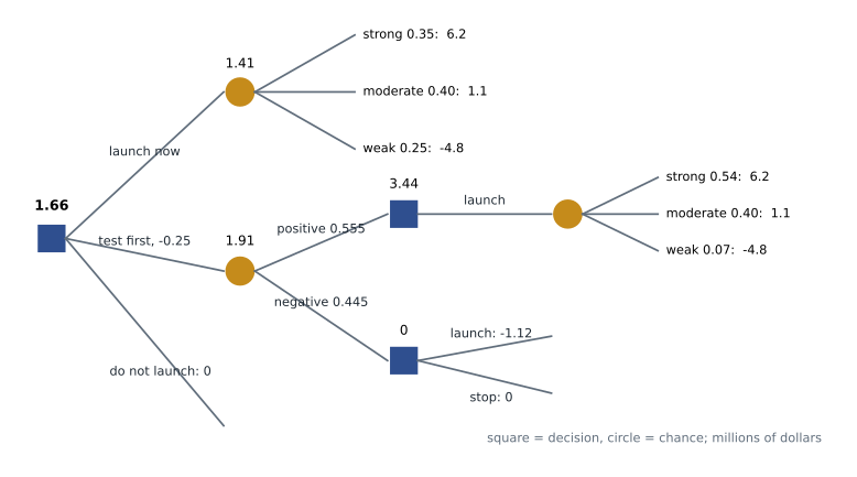
A decision tree lays out a sequence of decisions and uncertain events from left to right. Square nodes represent decisions, where management chooses a branch. Circular nodes represent chance events, where the branch is determined by uncertainty, with a probability on each branch. Outcomes are written at the right-hand end of each path. The tree is solved from right to left, a process called rolling back: at each chance node, calculate the expected value of its branches; at each decision node, choose the branch with the highest expected value.
GrainSense offers more than a launch-or-not choice. Northgate could first run a market test, selling the kit through 25 dealers in two regions for one season, at a cost of 250,000 dollars. The test would not reveal the true state of the market, but it would give a signal: a positive or negative result. Past tests of comparable agricultural technology suggest a positive result in about 85 percent of cases when the market turned out strong, 55 percent when it was moderate, and 15 percent when it was weak. After the test, Northgate would decide whether to launch.
Revising probabilities with Bayes' rule
To value the test, the tree needs the probability of each result and the revised probabilities of each market state after each result. Bayes' rule provides them. The probability of a positive result is the sum, over the three states, of the prior probability of the state times the probability of a positive result in that state. The posterior probability of a state given a positive result is the prior times the likelihood, divided by the probability of a positive result.
# Decision tree: launch the GrainSense sensor kit now, test the market first, or do not launch.
# NPVs in millions of dollars; probabilities are management estimates (invented).
states = ['strong', 'moderate', 'weak']
prior = {'strong': 0.35, 'moderate': 0.40, 'weak': 0.25}
npv_launch = {'strong': 6.2, 'moderate': 1.1, 'weak': -4.8}
test_cost = 0.25
# reliability of the market test: P(positive result | true state)
p_pos = {'strong': 0.85, 'moderate': 0.55, 'weak': 0.15}

ev_launch = sum(prior[s] * npv_launch[s] for s in states)
print(f"EV of launching now:       {ev_launch:6.3f}")
print(f"EV of not launching:       {0:6.3f}")
# perfect information: launch only in states where the NPV is positive
ev_perfect = sum(prior[s] * max(npv_launch[s], 0) for s in states)
evpi = ev_perfect - max(ev_launch, 0)
print(f"EV with perfect information: {ev_perfect:6.3f}  EVPI = {evpi:.3f}")
# market test: revise probabilities with Bayes' rule
ev_test = 0.0
for result in ('positive', 'negative'):
    like = {s: p_pos[s] if result == 'positive' else 1 - p_pos[s] for s in states}
    p_result = sum(prior[s] * like[s] for s in states)
    post = {s: prior[s] * like[s] / p_result for s in states}
    ev_if_launch = sum(post[s] * npv_launch[s] for s in states)
    best = max(ev_if_launch, 0)
    ev_test += p_result * best
    print(f"Test {result:8s}: P = {p_result:.3f}  posterior " +
          ', '.join(f"{s} {post[s]:.2f}" for s in states) +
          f"  EV if launch {ev_if_launch:6.3f} -> {'launch' if ev_if_launch > 0 else 'stop'}")
evsi = ev_test - max(ev_launch, 0)
print(f"EV with test (before its cost): {ev_test:6.3f}  EVSI = {evsi:.3f}")
print(f"Net value of testing: {evsi - test_cost:+.3f} -> {'test first' if evsi > test_cost else 'decide now'}")EV of launching now: 1.410 EV of not launching: 0.000 EV with perfect information: 2.610 EVPI = 1.200 Test positive: P = 0.555 posterior strong 0.54, moderate 0.40, weak 0.07 EV if launch 3.435 -> launch Test negative: P = 0.445 posterior strong 0.12, moderate 0.40, weak 0.48 EV if launch -1.116 -> stop EV with test (before its cost): 1.907 EVSI = 0.497 Net value of testing: +0.247 -> test first
The calculations show how informative the test is. A positive result, expected 55.5 percent of the time, raises the probability of a strong market from 35 to 54 percent and cuts the probability of a weak one from 25 to 7 percent. Launching after a positive result has an expected value of 3.44 million. A negative result raises the probability of a weak market to 48 percent, and launching would then have an expected value of −1.12 million, so Northgate would stop. Rolling back, the expected value of the test strategy before its cost is 1.91 million.
The value of information
The expected value of perfect information (EVPI) is the most a decision maker should pay to learn the true state before deciding. With perfect information, Northgate would launch in the strong and moderate states and not launch in the weak state, so the expected value would be 0.35 × 6.2 + 0.40 × 1.1 + 0.25 × 0 = 2.61 million. Without information, the best choice is to launch, worth 1.41 million. The difference, 1.20 million, is the EVPI. No research, however good, can be worth more than that.
The expected value of sample information (EVSI) is the value of an imperfect signal such as the market test. It equals the expected value with the test, 1.91 million before its cost, less the expected value without it, 1.41 million: 0.50 million. Because the test costs 0.25 million, its net value is about 0.25 million, so testing first is the better strategy. The ratio of EVSI to EVPI, about 41 percent, measures how much of the possible value of information the test captures. A more reliable test would capture more.
| Strategy | Expected value (millions) | Chance of a loss on launch | Comment |
|---|---|---|---|
| Launch now | 1.41 | 25% | Highest risk |
| Test first, then decide | 1.66 (after test cost) | About 4% | Best expected value, lower risk, one season's delay |
| Do not launch | 0 | 0% | Gives up the opportunity |
| With perfect information | 2.61 | 0% | Upper bound; EVPI is 1.20 |
Sensitivity analysis
The probabilities and NPVs in the tree are estimates. Sensitivity analysis asks how much they would have to change before the recommended decision changes. The probability of a weak market is the most uncertain input and the most consequential, so Grace varies it while holding the other estimates in proportion.
# Sensitivity and risk profile for the GrainSense decision (same invented data as before).
npv = {'strong': 6.2, 'moderate': 1.1, 'weak': -4.8}
p_pos = {'strong': 0.85, 'moderate': 0.55, 'weak': 0.15}
test_cost = 0.25

def values(p_weak):
    # hold the strong:moderate ratio at 35:40 while varying the chance of a weak market
    rest = 1 - p_weak
    prior = {'strong': rest * 35 / 75, 'moderate': rest * 40 / 75, 'weak': p_weak}
    launch = sum(prior[s] * npv[s] for s in npv)
    test = -test_cost
    for pos in (True, False):
        like = {s: p_pos[s] if pos else 1 - p_pos[s] for s in npv}
        pr = sum(prior[s] * like[s] for s in npv)
        test += max(sum(prior[s] * like[s] * npv[s] for s in npv) / pr, 0) * pr
    return launch, test

print('P(weak)  launch now  test first  best choice')
for pw in (0.10, 0.20, 0.25, 0.30, 0.40, 0.50):
    l, t = values(pw)
    best = max((l, 'launch now'), (t, 'test first'), (0.0, 'do not launch'))[1]
    print(f"  {pw:.2f}    {l:7.3f}     {t:7.3f}    {best}")
# risk profile: chance of losing money under each strategy at the base estimate (0.25)
prior = {'strong': 0.35, 'moderate': 0.40, 'weak': 0.25}
p_loss_launch = prior['weak']
p_loss_test = prior['weak'] * p_pos['weak']    # launch after a positive test in a weak market
print(f"P(launch loses money): launch now {p_loss_launch:.3f}, test first {p_loss_test:.3f}")P(weak) launch now test first best choice 0.10 2.652 2.402 launch now 0.20 1.824 1.832 test first 0.25 1.410 1.657 test first 0.30 0.996 1.481 test first 0.40 0.168 1.131 test first 0.50 -0.660 0.781 test first P(launch loses money): launch now 0.250, test first 0.037
The test-first strategy is best for any probability of a weak market from about 0.20 upward; only if management were confident the weak market had a probability around 0.10 would launching immediately be better. Even when the weak market is as likely as not, testing keeps the expected value positive, because the test lets Northgate avoid most of the downside. The risk profile shows the same thing from another angle: the probability that a launch ends in the weak market falls from 25 percent if Northgate launches now to under 4 percent if it tests first and launches only after a positive result. The cost of this protection is the 0.25 million test and a one-season delay, which a fuller analysis might value through the risk that a competitor reaches the market first.
Worked problem
Break-even probability
Ignoring the test, at what probability of a weak market would launching now have an expected value of zero, if the strong and moderate states keep their 35:40 ratio?
Show solution
- Let w be the probability of a weak market. Then the strong market has probability (1 − w) × 35/75 and the moderate market (1 − w) × 40/75.
- The expected value is (1 − w)(35 × 6.2 + 40 × 1.1)/75 − 4.8w = (1 − w)(3.48) − 4.8w.
- Setting this to zero: 3.48 = 8.28w, so w ≈ 0.42.
Answer: About 0.42: launching now has a positive expected value as long as the weak market is less likely than about 42 percent.
Attitudes to risk
Expected value treats a certain 1 million and a 50 percent chance of 2 million as equally good. Most people and most organizations are risk averse: they prefer the certain million. Utility theory captures this by converting monetary outcomes into utilities with a concave function, so that each extra dollar adds less utility than the last, and choosing the alternative with the highest expected utility. The certainty equivalent of a risky alternative is the sure amount that gives the same utility; the difference between the expected value and the certainty equivalent is the risk premium.
Utility functions are hard to elicit in practice, so organizations usually handle risk aversion more informally: by setting limits on the maximum acceptable loss, by requiring higher returns on riskier projects, or by preferring strategies, like the market test, that reduce the spread of outcomes even at some cost. Simple decision rules for complete uncertainty, such as maximin (choose the alternative whose worst outcome is best) and minimax regret (choose the alternative that minimizes the largest regret across states), are sometimes taught as alternatives. They can be useful as checks, but they ignore probabilities entirely and can lead to very cautious choices.
| Rule | How it works | GrainSense choice |
|---|---|---|
| Expected value | Maximize the probability-weighted average | Test first (1.66 after cost) |
| Maximin | Maximize the worst outcome | Do not launch (worst outcome 0) |
| Maximax | Maximize the best outcome | Launch now (best outcome 6.2) |
| Minimax regret | Minimize the largest regret | Test first (largest regret about 1.18 million) |
| Expected utility | Maximize probability-weighted utility | Depends on the utility function; risk aversion favors testing |
Behavioral traps
Decision analysis is only as good as the probabilities and values that go into it, and behavioral research has documented systematic biases in how people estimate them. Overconfidence leads to probability ranges that are too narrow: in studies where experts give 90 percent confidence intervals, the true value often falls outside them far more than 10 percent of the time. Anchoring leads estimates to stay close to an initial number, such as last year's sales or the first figure mentioned in a meeting. The planning fallacy, identified by Daniel Kahneman and Amos Tversky, describes the tendency to underestimate costs and completion times for one's own projects. Confirmation bias leads people to seek evidence that supports their preferred option.
Several practices reduce these biases. Reference class forecasting, recommended by Kahneman and developed by Bent Flyvbjerg, starts from the actual outcomes of a set of similar past projects rather than from the specifics of the current one. A pre-mortem asks the team to imagine that the project has failed and to explain why, which surfaces risks that optimism hides. Assigning someone the role of challenging the analysis, and recording probability estimates so that they can be compared with outcomes, both help. At Northgate, the product team's first estimate gave the weak market a probability of 10 percent; using outcomes from comparable agricultural technology launches as a reference class raised it to 25 percent, which changed the recommended decision from launch now to test first.
Common mistakes
MistakeUsing expected value alone for a large, one-off bet.
InsteadConsider the spread of outcomes, the chance of a loss and the organization's capacity to absorb it.
MistakeTreating a market test result as revealing the true state.
InsteadUse Bayes' rule to revise probabilities; tests give imperfect signals.
MistakePaying more for research than the EVPI.
InsteadEVPI is the upper bound on the value of any information.
MistakePresenting one set of probabilities as fact.
InsteadShow how the decision changes as key probabilities vary.
MistakeAccepting the project team's probability estimates without challenge.
InsteadUse reference classes, pre-mortems and recorded estimates to counter optimism.
Summary and key terms
- Business decisions usually rely on subjective probabilities that should be consistent with evidence and revised as it arrives.
- Expected value is the probability-weighted average of outcomes; launching GrainSense now has an expected value of 1.41 million.
- Decision trees are solved by rolling back: expected values at chance nodes, best choices at decision nodes.
- Bayes' rule revises probabilities after a test; a positive GrainSense test raises the chance of a strong market from 35% to 54%.
- EVPI, 1.20 million here, caps the value of any information; EVSI for the market test is 0.50 million against a cost of 0.25 million.
- Testing first is the best strategy for any probability of a weak market above about 0.20.
- Risk aversion can be modeled with utility, or handled through loss limits and risk-reducing strategies.
- Overconfidence, anchoring and the planning fallacy distort estimates; reference classes and pre-mortems help.
- Expected value
- The probability-weighted average of the possible outcomes of an alternative.
- Decision tree
- A diagram of decisions, chance events, probabilities and outcomes, solved from right to left.
- Rolling back
- Solving a decision tree by computing expected values at chance nodes and choosing the best branch at decision nodes.
- Bayes' rule
- A formula for revising probabilities in light of new evidence.
- Expected value of perfect information (EVPI)
- The increase in expected value from knowing the true state before deciding.
- Expected value of sample information (EVSI)
- The increase in expected value from an imperfect signal such as a test.
- Certainty equivalent
- The sure amount a decision maker values as highly as a risky alternative.
- Reference class forecasting
- Forecasting from the actual outcomes of a group of similar past projects.
- Pre-mortem
- An exercise in which a team imagines a project has failed and explains why.
Practice problems
Work each problem on paper first, then reveal the answer to check.
Calculate the expected value of launching GrainSense now.
Show answer
0.35 × 6.2 + 0.40 × 1.1 + 0.25 × (−4.8) = 1.41 million.
What is the EVPI, and what does it tell management?
Show answer
1.20 million; no information can be worth more than that.
What is the probability of a positive test result?
Show answer
0.555.
After a negative test, what is the probability of a weak market?
Show answer
About 0.48.
Change the test cost in the program to 0.6 million. What should Northgate do?
Show answer
Launch now, because EVSI of about 0.50 is less than the test cost.
Change P(positive | weak) to 0.40. What happens to EVSI?
Show answer
It falls to about 0.20 million, below the test cost, because the test is less able to distinguish a weak market.
Why might expected value be inappropriate for a single very large investment?
Show answer
Outcomes will not average out, and a large loss could threaten the organization.
What decision does the maximin rule recommend for GrainSense, and why is it of limited use?
Show answer
Do not launch; it ignores probabilities and is extremely cautious.
How did reference class forecasting change the GrainSense recommendation?
Show answer
It raised the weak-market probability from 10% to 25%, making testing first the best strategy.
What is a pre-mortem?
Show answer
An exercise imagining that the project has failed and explaining why, to surface hidden risks.
Lesson quiz · 5 questions
Score 60% or more to complete this lesson.
Create a free account to save your progress, take quizzes and earn a certificate.