
ACCT-222 · Lesson 8 of 12 · 29 min
Standard costing I: setting standards and direct-cost variances
A standard cost is a carefully predetermined cost of one unit of output: how much of each input should be used and what each unit of input should cost. ACCT-102 lesson 11 introduced flexible budgets and the basic price and efficiency variances for direct materials and direct labor. This lesson and the next two develop standard costing in more depth. Here we look at how standards are set, at the choice between ideal and attainable standards, at when to measure the materials price variance, and at mix and yield variances, which split the efficiency variance when several inputs can be substituted for one another. Lesson 9 covers overhead variances and the journal entries of a standard cost system, and lesson 10 turns to sales variances.
Why companies use standard costs
Standard costs serve several purposes at once. They provide benchmarks for evaluating performance, so that managers can focus on significant departures from plan. They simplify bookkeeping, because inventory can be carried at standard cost and the differences recorded in variance accounts. They support pricing and bidding, because the standard cost of a new order can be estimated quickly from the standard bills of materials and routings. And they make budgeting easier, because the budget for any level of output is simply standard cost per unit multiplied by planned units.
Standard costing is sometimes described as old-fashioned, suited to labor-intensive mass production rather than to automated, flexible or service operations. There is some truth in the criticism: in a plant where direct labor is 5 percent of cost, detailed labor variances matter little, and monthly variance reports arrive too late to guide shop-floor decisions that are made by the hour. But surveys continue to find standard costing in wide use, especially in process industries, food, chemicals and metals, where materials dominate and yields matter. The tool has adapted: modern systems compute variances daily, focus on materials and yields rather than labor, and pair the financial variances with non-financial measures such as scrap rates and first-pass yield.
Setting standards
A standard has a quantity part and a price part. For direct materials, the standard quantity per unit comes from engineering specifications (the bill of materials), adjusted for unavoidable waste, evaporation or shrinkage. The standard price is the expected purchase cost per unit of material, including freight and handling and net of expected discounts. For direct labor, the standard hours per unit come from time-and-motion studies or historical data (the routing), adjusted for unavoidable breaks, set-ups and rejects. The standard rate is the expected wage rate including payroll taxes and benefits where the company treats them as part of direct labor.
Setting standards is a joint effort. Purchasing proposes materials prices, engineering proposes quantities, production supervisors and human resources advise on labor hours and rates, and accounting assembles the standard cost card. The participation matters: managers are more likely to accept standards they helped set, and they bring knowledge the accountant does not have.
| Input | Standard quantity per pump | Standard price | Standard cost per pump |
|---|---|---|---|
| Cast iron | 8 kg | $1.20 per kg | $9.60 |
| Nickel alloy | 2 kg | $6.00 per kg | $12.00 |
| Senior assembly technician | 0.4 hours | $42 per hour | $16.80 |
| Junior assembly technician | 0.6 hours | $26 per hour | $15.60 |
| Total direct cost of the housing and assembly steps | $54.00 |
Ideal versus attainable standards
Ideal standards assume perfect operating conditions: no waste, no breakdowns, no idle time, every worker at peak efficiency. Currently attainable standards allow for normal waste, normal machine downtime and normal worker fatigue; they are demanding but achievable by a skilled, motivated team. Most companies use currently attainable standards. Ideal standards produce unfavorable variances every month, which become routine and are ignored, and they can discourage employees who see the target as impossible. Attainable standards produce variances that mean something: a favorable variance signals genuinely good performance, and an unfavorable variance signals a problem worth investigating.
Companies that pursue continuous improvement sometimes use a third approach: standards that tighten each period, built into kaizen budgets, so that the target moves as the process improves. Whatever the approach, standards should be reviewed at least annually and whenever a significant change in materials, methods or prices occurs. Stale standards, set years ago and never updated, are one of the commonest reasons standard costing loses credibility.
The basic variances revisited
For each direct input, the total flexible-budget variance (actual cost minus the standard cost allowed for the actual output) splits into a price variance and an efficiency (quantity) variance. Using AQ for actual quantity, AP for actual price, SQ for the standard quantity allowed for actual output and SP for the standard price:
A positive result means actual cost exceeded standard and the variance is unfavorable (U); a negative result is favorable (F). In October Halden produced 1,800 S-100 housings. Purchasing bought and the foundry used 15,600 kg of cast iron at $1.25 per kg and 4,200 kg of nickel alloy at $5.80 per kg. The assembly line worked 760 senior technician hours at $43 and 1,100 junior technician hours at $25.50.
# Direct materials and direct-hour price and efficiency variances, October (illustrative)
output = 1_800
materials = {   # name: (std qty per unit, std price, actual qty, actual price)
    "cast iron":    (8, 1.20, 15_600, 1.25),
    "nickel alloy": (2, 6.00, 4_200, 5.80),
}
crew = {
    "senior": (0.4, 42.0, 760, 43.0),
    "junior": (0.6, 26.0, 1_100, 25.5),
}

def variances(inputs, label):
    tp = te = 0
    for name, (sq_u, sp, aq, ap) in inputs.items():
        sq = sq_u * output
        price = (ap - sp) * aq
        eff = (aq - sq) * sp
        tp += price; te += eff
        print(f"{label} {name:<13} SQ {sq:>7,.0f}  price {price:>+8,.0f}  efficiency {eff:>+8,.0f}")
    print(f"{label} total price {tp:+,.0f}   total efficiency {te:+,.0f}   (+ = U, - = F)")

variances(materials, "DM")
variances(crew, "DL")DM cast iron SQ 14,400 price +780 efficiency +1,440 DM nickel alloy SQ 3,600 price -840 efficiency +3,600 DM total price -60 total efficiency +5,040 (+ = U, - = F) DL senior SQ 720 price +760 efficiency +1,680 DL junior SQ 1,080 price -550 efficiency +520 DL total price +210 total efficiency +2,200 (+ = U, - = F)
For materials, the price variances nearly offset each other: cast iron cost $780 more than standard, while nickel alloy cost $840 less, for a net $60 favorable. The efficiency variances, however, total $5,040 unfavorable, because the foundry used 19,800 kg of alloy in total against a standard of 18,000 kg for the castings produced. For labor, the rate variance is a modest $210 unfavorable (seniors paid $1 above standard, juniors $0.50 below), but the efficiency variance is $2,200 unfavorable because the line used 1,860 hours against a standard of 1,800.
When to record the materials price variance
The materials price variance can be measured when materials are purchased or when they are used. Measuring it at purchase is generally preferred. It gives purchasing managers timely feedback on the decisions they control, it allows materials inventory to be carried at standard price (which simplifies record-keeping), and it avoids the delay that occurs when materials sit in inventory for months before use. Measuring it at use defers the variance until the materials enter production, which can hide purchasing problems for a long time.
In October Halden bought exactly what it used, so the timing does not matter. In November, purchasing took advantage of a volume discount and bought 30,000 kg of cast iron at $1.14 per kg, of which only 14,500 kg was used. Measured at purchase, the price variance is (1.14 − 1.20) × 30,000 = $1,800 favorable, reported in November; measured at use, only (1.14 − 1.20) × 14,500 = $870 favorable would be reported in November, with the rest appearing as the iron is used. The large purchase also raises a question the price variance alone does not answer: did the discount justify the cost of holding 15,500 kg of extra inventory? A favorable price variance can hide carrying costs, storage space and the risk of obsolescence.
Mix and yield variances
When a product uses several inputs that can be substituted for one another within limits, the efficiency variance can be split further. Halden's foundry blends cast iron and nickel alloy in a standard ratio of 80:20 by weight. The metallurgist can vary the blend somewhat: more nickel alloy improves corrosion resistance and reduces cracking, but nickel alloy costs five times as much as iron. The efficiency variance then has two causes. The mix variance measures the effect of using a different blend from standard. The yield variance measures the effect of using more or less total input than standard for the output achieved.
To separate them, compute the actual total quantity of all inputs used, apply the standard mix to it, and compare. The mix variance compares the actual quantities with the actual total at standard mix, both valued at standard prices. The yield variance compares the actual total at standard mix with the standard quantities allowed for actual output, valued at standard prices.
Here m_i is input i's standard share of the mix. Together the mix and yield variances add up to the total efficiency variance.
# Mix and yield variances for the foundry blend and the assembly crew (illustrative)
output = 1_800

def mix_yield(inputs, label):
    total_actual = sum(aq for _, _, aq in inputs.values())
    std_total_per_unit = sum(q for q, _, _ in inputs.values())
    mix_v = yield_v = 0
    for name, (q_u, sp, aq) in inputs.items():
        share = q_u / std_total_per_unit
        at_std_mix = total_actual * share
        sq = q_u * output
        mix_v += sp * (aq - at_std_mix)
        yield_v += sp * (at_std_mix - sq)
        print(f"{label} {name:<13} actual {aq:>7,}  actual total at std mix {at_std_mix:>8,.0f}  SQ {sq:>7,.0f}")
    print(f"{label} mix variance {mix_v:+,.0f}   yield variance {yield_v:+,.0f}   "
          f"sum {mix_v + yield_v:+,.0f}   (+ = U, - = F)")

mix_yield({"cast iron": (8, 1.20, 15_600), "nickel alloy": (2, 6.00, 4_200)}, "DM")
mix_yield({"senior": (0.4, 42.0, 760), "junior": (0.6, 26.0, 1_100)}, "DL")DM cast iron actual 15,600 actual total at std mix 15,840 SQ 14,400 DM nickel alloy actual 4,200 actual total at std mix 3,960 SQ 3,600 DM mix variance +1,152 yield variance +3,888 sum +5,040 (+ = U, - = F) DL senior actual 760 actual total at std mix 744 SQ 720 DL junior actual 1,100 actual total at std mix 1,116 SQ 1,080 DL mix variance +256 yield variance +1,944 sum +2,200 (+ = U, - = F)
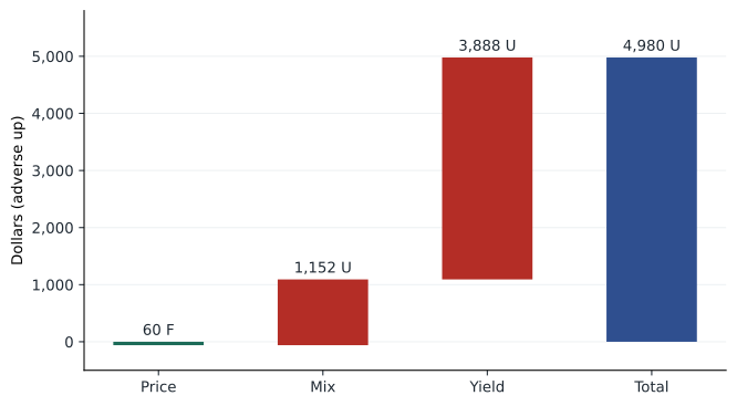
For the foundry, the actual blend used 4,200 kg of nickel alloy out of 19,800 kg, about 21.2 percent instead of the standard 20 percent. At the standard mix, the 19,800 kg would have contained 15,840 kg of iron and 3,960 kg of nickel alloy. Using more of the expensive input produced a mix variance of $1,152 unfavorable. The yield variance, $3,888 unfavorable, shows the larger problem: the foundry needed 19,800 kg of input to produce castings that should have needed 18,000 kg, about 10 percent more than standard. The materials efficiency variance of $5,040 is the sum of the two.
For the assembly line, the labor mix variance is $256 unfavorable (slightly more senior hours than the 40:60 standard), and the yield variance, $1,944 unfavorable, shows that the crew needed 60 more hours than standard in total for the pumps produced.
Interpreting mix and yield together
Mix and yield variances often move in opposite directions, and interpreting them requires talking to the people who make the decisions. The metallurgist's explanation in October was that a batch of cast iron from a new supplier had higher sulfur content, which caused cracking, so she raised the nickel share to compensate. That decision cost $1,152 in mix. It did not prevent the yield problem: many castings still cracked and had to be remelted, which consumed extra metal. The purchasing manager, meanwhile, had a slightly unfavorable price variance on iron because the new supplier's price was higher than standard as well. The variances together point to the new iron supplier as the root cause, which the separate price, mix and yield figures alone could not show.
A favorable mix variance is not automatically good news either. If the foundry had cut the nickel share to 15 percent to save money, it would have reported a favorable mix variance, but more castings might have cracked, producing an unfavorable yield variance and, worse, more pumps failing in the field. Mix decisions should be judged by their effect on total cost and quality, not by the mix variance alone.
Labor variances in a modern plant
Labor efficiency variances assume labor hours vary with output. In many plants they do not: assembly crews are scheduled for full shifts, and if demand falls, workers are reassigned to cleaning, training or maintenance rather than sent home. In that setting, an unfavorable labor efficiency variance may simply reflect a slow month rather than poor productivity, and pressing supervisors to eliminate it can encourage overproduction to keep workers busy, building inventory nobody ordered. Lean plants often replace labor efficiency variances with measures such as units per labor hour on the bottleneck, on-time delivery and first-pass yield, and treat direct labor as a fixed cost of capacity.
The labor mix variance remains useful where crews combine workers of different skill levels and pay rates. Halden's assembly standard of 40 percent senior and 60 percent junior hours reflects the work's skill requirements. A crew that relies too heavily on seniors costs more; one that relies too heavily on juniors may produce more defects and rework, which would show up later as spoilage costs and warranty claims.
Deciding which variances to investigate
Variances are signals, not verdicts. Managers cannot investigate every variance, so they use management by exception, investigating those that are large in absolute terms, large relative to standard, recurring, or trending in one direction. Statistical process control charts can help distinguish random fluctuations from genuine shifts. The cost of an investigation should be weighed against the expected benefit of correcting a problem: a variance of $500 in a month is unlikely to justify a week of engineering time, unless it is the first sign of a trend that will grow.
Worked problem
A simple investigation rule
Halden investigates any materials variance that exceeds 5 percent of the standard cost allowed or $3,000, whichever is lower. The standard materials cost allowed for October's output was 14,400 kg of iron at $1.20 plus 3,600 kg of nickel alloy at $6.00. Which October materials variances should be investigated?
Show solution
- Standard cost allowed = $17,280 + $21,600 = $38,880; 5 percent = $1,944. The threshold is the lower of $1,944 and $3,000, which is $1,944.
- Net price variance $60 F: no investigation.
- Mix variance $1,152 U: below threshold, but note it in the report.
- Yield variance $3,888 U: above threshold; investigate.
Answer: Investigate the yield variance; the investigation leads to the new iron supplier.
Common mistakes
MistakeUsing ideal standards and expecting them to motivate.
InsteadUse currently attainable standards so variances carry meaning.
MistakeMeasuring the materials price variance only when materials are used.
InsteadMeasure it at purchase for timely feedback, and check whether bulk-buying savings exceed carrying costs.
MistakeTreating a favorable mix variance as good news on its own.
InsteadRead mix and yield variances together and consider quality effects.
MistakeComputing efficiency variances with budgeted output rather than actual output.
InsteadBase standard quantities on the actual output produced.
MistakeAssuming labor efficiency variances always measure productivity.
InsteadWhen labor is fixed in the short run, the variance may reflect volume; use non-financial measures too.
Summary and key terms
- Standard costs predetermine the quantity and price of each input per unit of output.
- Standards come from engineering, purchasing, production and accounting working together, and should be reviewed regularly.
- Currently attainable standards are preferred to ideal standards.
- Price variance = (AP − SP) × AQ; efficiency variance = (AQ − SQ) × SP, with SQ based on actual output.
- The materials price variance is best measured at purchase.
- When inputs can be substituted, the efficiency variance splits into mix and yield variances.
- Variances are signals to investigate selectively, interpreted together with operating information.
- Standard cost
- A carefully predetermined cost of one unit of output.
- Currently attainable standard
- A standard achievable under efficient operating conditions with normal waste and downtime.
- Ideal standard
- A standard assuming perfect conditions with no waste or downtime.
- Price variance
- The difference between actual and standard price multiplied by actual quantity.
- Efficiency variance
- The difference between actual and standard quantity for actual output, at standard price.
- Mix variance
- The effect on cost of using a different proportion of inputs from the standard mix.
- Yield variance
- The effect on cost of using a different total quantity of inputs from standard for actual output.
- Standard cost card
- A record of the standard quantities and prices of each input for one unit of output.
- Management by exception
- Focusing attention on significant departures from plan.
- Kaizen budgeting
- Budgeting that builds continuous improvement into each period's targets.
Practice problems
Work each problem on paper first, then reveal the answer to check.
A plant uses 5,200 kg of material at $3.10 per kg; the standard is 2.5 kg per unit at $3.00, and 2,000 units are made. Compute the price and efficiency variances.
Show answer
Price $520 U; efficiency (5,200 − 5,000) × $3 = $600 U.
Labor: 3,150 hours at $28.60; standard 1.5 hours per unit at $28; 2,000 units. Compute the rate and efficiency variances.
Show answer
Rate $1,890 U; efficiency (3,150 − 3,000) × $28 = $4,200 U.
Inputs X (std 60%, $4/kg) and Y (std 40%, $9/kg); standard 10 kg per unit; 500 units made; actual X 3,300 kg, Y 2,100 kg. Compute the mix variance.
Show answer
Actual total 5,400 at std mix: X 3,240, Y 2,160. Mix = 4 × 60 + 9 × (−60) = $300 F.
Compute the yield variance for the previous question.
Show answer
SQ: X 3,000, Y 2,000. Yield = 4 × 240 + 9 × 160 = $2,400 U.
Check that mix plus yield equals the efficiency variance in the previous two questions.
Show answer
Efficiency = 4 × 300 + 9 × 100 = $2,100 U = $300 F + $2,400 U.
In November Halden bought 30,000 kg of iron at $1.14. What price variance is recorded at purchase?
Show answer
$1,800 F.
Give two reasons to prefer currently attainable standards.
Show answer
Variances become meaningful signals; employees accept achievable targets and stay motivated.
Why might a favorable labor mix variance be bad news?
Show answer
Using more junior hours may raise defects, rework and warranty costs.
What does a yield variance of 10 percent more input than standard suggest in the foundry?
Show answer
Cracking, remelting or other losses; investigate materials quality and process settings.
Why might a lean plant drop labor efficiency variances?
Show answer
Labor is effectively fixed, and the variance can encourage overproduction to absorb hours.
Lesson quiz · 5 questions
Score 60% or more to complete this lesson.
Create a free account to save your progress, take quizzes and earn a certificate.