
ACCT-222 · Lesson 4 of 12 · 27 min
Activity-based costing and activity-based management
ACCT-102 lesson 7 introduced activity-based costing (ABC) as a way to assign overhead using activities rather than a single volume-based measure. This lesson builds a full ABC system for Halden's manufacturing division, compares it in detail with plantwide and departmental rates, and then turns to activity-based management: using activity information to reduce cost rather than merely measure it. The central idea is simple. Products do not consume overhead directly; they consume activities, and activities consume resources. If we can identify the significant activities, measure what drives each one, and trace activity costs to products in proportion to their use of those drivers, product costs will reflect how the products actually use the plant.
Why volume-based rates distort costs
A plantwide rate based on direct labor hours assumes that every overhead cost rises in proportion to labor hours. Some overhead does behave that way: electricity for hand tools, supervision of assembly workers, payroll processing. Much does not. The cost of setting up a machine depends on how many batches are run, not how many units are in each batch. The cost of engineering change orders depends on how many product designs must be maintained and how often they change. The cost of the plant building depends on the size of the facility. When these costs are assigned by labor hours, high-volume products with large batches and stable designs subsidize low-volume products with small batches and frequent changes. This is known as product-cost cross-subsidization.
Halden illustrates the problem sharply. The S-100 is made in batches of 500, its design changes rarely, and it is inspected on a sampling basis. The C-900 is made in batches of five, each batch needs engineering attention, and every pump is fully inspected. Yet under the plantwide rate the C-900 receives only six times the overhead of an S-100 per unit, because it uses six times the labor.
The cost hierarchy
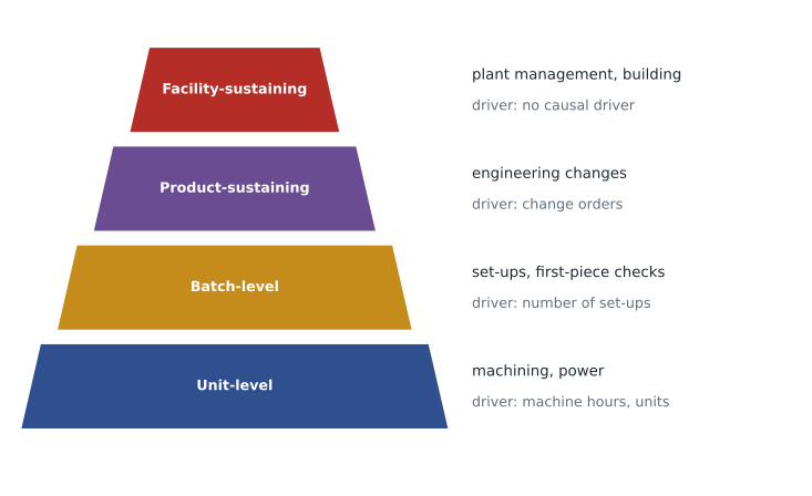
ABC classifies activities by the level at which they are performed. The cost hierarchy has four levels:
- Unit-level activities are performed on each unit, so their cost varies with units produced: running a machine, inserting a component, unit-level power.
- Batch-level activities are performed for each batch, regardless of its size: setting up machines, issuing material for a production run, first-piece inspection.
- Product-sustaining activities support a product line regardless of how many units or batches are made: engineering design, maintaining bills of materials, engineering change orders.
- Facility-sustaining activities keep the plant running and cannot be traced to products by any cause-and-effect driver: plant management, building depreciation, property taxes, security.
The hierarchy explains why volume-based rates fail: only unit-level costs vary with volume. Batch, product and facility costs are driven by other things. Many ABC designers do not allocate facility-sustaining costs to products at all for decision purposes, because any allocation is arbitrary; they deduct them from total product margins as a lump sum. For inventory valuation, which requires full absorption of manufacturing overhead, they are usually spread with a simple base such as labor hours or machine hours.
Building Halden's ABC system
An ABC project follows a standard sequence. First, identify the main activities, usually through interviews with supervisors and support staff and by analyzing how people spend their time. Second, assign resource costs (salaries, depreciation, supplies) to activity cost pools, often using percentage-of-time estimates for shared staff. Third, choose a cost driver for each activity that reflects what causes the activity's cost and that can be measured economically. Fourth, compute an activity rate for each pool by dividing pool cost by the total quantity of the driver. Fifth, assign activity costs to products by multiplying each activity rate by the quantity of the driver each product uses.
| Activity pool | Level | Annual cost | Driver | Total driver quantity |
|---|---|---|---|---|
| Machining | Unit | $600,000 | Machine hours | 20,000 |
| Set-ups | Batch | $300,000 | Number of set-ups | 200 |
| Engineering support | Product-sustaining | $350,000 | Engineering change orders | 70 |
| Quality inspection | Batch and unit | $200,000 | Inspection hours | 4,000 |
| Facility | Facility-sustaining | $200,000 | Direct labor hours (for inventory only) | 33,000 |
| Total | $1,650,000 |
| Driver use | S-100 | P-300 | C-900 | Total |
|---|---|---|---|---|
| Machine hours | 10,000 | 7,500 | 2,500 | 20,000 |
| Set-ups | 40 | 60 | 100 | 200 |
| Engineering change orders | 10 | 20 | 40 | 70 |
| Inspection hours | 1,000 | 1,500 | 1,500 | 4,000 |
| Direct labor hours | 20,000 | 10,000 | 3,000 | 33,000 |
The driver data already reveal the pattern. The S-100 makes 78 percent of the units (20,000 of 25,500) but uses only 20 percent of the set-ups and 14 percent of the engineering change orders. The C-900 makes 2 percent of the units but uses half of the set-ups and more than half of the engineering changes.
# Halden manufacturing division: plantwide rate versus ABC (illustrative)
units = {"S-100": 20_000, "P-300": 5_000, "C-900": 500}
pools = {   # cost, driver use by S-100, P-300, C-900
    "Machining":   (600_000, (10_000, 7_500, 2_500)),
    "Set-ups":     (300_000, (40, 60, 100)),
    "Engineering": (350_000, (10, 20, 40)),
    "Inspection":  (200_000, (1_000, 1_500, 1_500)),
    "Facility":    (200_000, (20_000, 10_000, 3_000)),
}
dlh = (20_000, 10_000, 3_000)
plantwide = sum(c for c, _ in pools.values()) / sum(dlh)

abc = [0.0, 0.0, 0.0]
for name, (cost, use) in pools.items():
    rate = cost / sum(use)
    print(f"{name:<12} rate {rate:>10,.2f} per driver unit")
    for i, q in enumerate(use):
        abc[i] += rate * q

print()
print(f"{'Product':<7}{'Plantwide OH/unit':>19}{'ABC OH/unit':>13}{'Change':>10}")
for i, p in enumerate(units):
    pw = plantwide * dlh[i] / units[p]
    a = abc[i] / units[p]
    print(f"{p:<7}{pw:>19,.2f}{a:>13,.2f}{a - pw:>+10,.2f}")
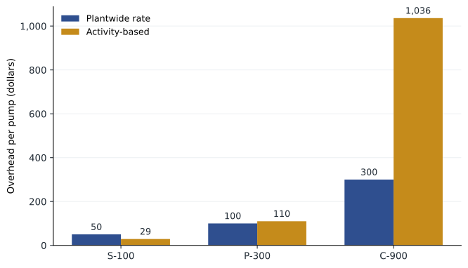
print(f"Total overhead assigned: {sum(abc):,.0f}")Machining rate 30.00 per driver unit Set-ups rate 1,500.00 per driver unit Engineering rate 5,000.00 per driver unit Inspection rate 50.00 per driver unit Facility rate 6.06 per driver unit Product Plantwide OH/unit ABC OH/unit Change S-100 50.00 29.06 -20.94 P-300 100.00 110.12 +10.12 C-900 300.00 1,036.36 +736.36 Total overhead assigned: 1,650,000
The activity rates are $30 per machine hour, $1,500 per set-up, $5,000 per engineering change order, $50 per inspection hour and about $6.06 per direct labor hour for facility costs. Under ABC, the S-100 carries about $29.06 of overhead per pump instead of $50.00; the P-300 carries about $110.12 instead of $100.00; and the C-900 carries about $1,036.36 instead of $300.00. Total overhead assigned is unchanged at $1,650,000. ABC does not create or remove cost; it redistributes the same cost according to how products use activities.
Departmental rates: a middle step
Before investing in ABC, many companies move from a plantwide rate to departmental rates. Halden could split its overhead into a machining department (machining, set-ups and half of inspection, $1,050,000, assigned by machine hours) and an assembly department (engineering, the other half of inspection and facility costs, $600,000, assigned by direct labor hours). Departmental rates recognize that the departments use different resources, but within each department they still assume all costs vary with one volume measure.
# Departmental rates for comparison (illustrative)
units = {"S-100": 20_000, "P-300": 5_000, "C-900": 500}
mh = (10_000, 7_500, 2_500)
dlh = (20_000, 10_000, 3_000)
machining_pool, assembly_pool = 1_050_000, 600_000
r_m = machining_pool / sum(mh)
r_a = assembly_pool / sum(dlh)
print(f"Machining rate ${r_m:.2f} per MH; assembly rate ${r_a:.2f} per DLH")
for i, p in enumerate(units):
    oh = (r_m * mh[i] + r_a * dlh[i]) / units[p]
print(f"{p}: departmental overhead per unit ${oh:,.2f}")Machining rate $52.50 per MH; assembly rate $18.18 per DLH S-100: departmental overhead per unit $44.43 P-300: departmental overhead per unit $115.11 C-900: departmental overhead per unit $371.59
Departmental rates move costs in the right direction (the S-100 falls to about $44.43 and the C-900 rises to about $371.59) but capture only a fraction of the distortion, because set-ups and engineering changes still ride on machine hours and labor hours. The comparison illustrates a general result: refining the cost system matters most when products differ in batch size, complexity and support needs, not just in how long they take to make.
| Overhead per unit | Plantwide | Departmental | Activity-based |
|---|---|---|---|
| S-100 | $50.00 | $44.43 | $29.06 |
| P-300 | $100.00 | $115.11 | $110.12 |
| C-900 | $300.00 | $371.59 | $1,036.36 |
What the new costs mean
Combining the ABC overhead with direct materials of $60, $140 and $520 and direct labor at $32 an hour gives full manufacturing costs of about $121 for the S-100, $314 for the P-300 and $1,748 for the C-900. Halden's list prices to dealers are $175, $390 and $1,650. Under the old system, the C-900 appeared to earn a gross margin of $638 per pump; under ABC it loses about $98 per pump before any selling or service costs. Meanwhile the S-100, which the old system said earned $33 per pump, actually earns about $54, enough to support a price cut that would help Halden compete in the residential market.
These results do not mean Halden should immediately stop making the C-900. Some of the C-900's activity costs, such as engineering salaries and set-up crews, will not disappear if the line is dropped unless the resources are actually removed or redeployed. Custom pumps may also bring in customers who buy other products, or keep Halden's engineering team sharp. But the analysis changes the conversation: it suggests the C-900 should be repriced, redesigned to need fewer engineering changes, made in larger batches, or offered only to customers willing to pay for customization. Lesson 5 extends the analysis beyond the factory to the cost of serving each customer.
Activity-based management
Activity-based management (ABM) uses ABC information to improve processes and reduce costs. Its first tool is value-added analysis. A value-added activity is one that customers perceive as adding usefulness and are willing to pay for, such as machining the impeller or assembling the motor. A non-value-added activity adds cost without adding customer value: moving parts between buildings, waiting for set-ups, inspecting to catch defects that a better process would not create, reworking failed units. Some non-value-added activities are necessary given the current process; the aim is to reduce or redesign them over time.
ABM also targets cost drivers. If set-ups cost $1,500 each, the way to reduce set-up cost is to reduce the number of set-ups (larger batches, fewer product variants, shared components) or to reduce the cost per set-up (quick-change tooling, standardized fixtures, set-up teams trained in single-minute exchange of die methods). If engineering change orders cost $5,000 each, the way to reduce them is to design products right the first time and to standardize parts across the range. BUS-230 lesson 11 describes these lean techniques from the operations side; ABC supplies the cost figures that justify them.
Worked problem
Valuing a set-up reduction project
Halden's operations team proposes quick-change fixtures for the machining centers, costing $90,000, which would cut set-up time and allow the set-up activity's cost to fall by 40 percent if one of the two set-up technicians is reassigned to the new P-300 cell, where a technician would otherwise be hired. Should Halden proceed?
Show solution
- Set-up activity cost is $300,000 a year; a 40 percent reduction is $120,000 a year in resources used.
- The saving is real only because the freed technician fills a position that would otherwise require a new hire. If the technician simply had idle time, the cost would not fall.
- Payback = $90,000 ÷ $120,000 ≈ 0.75 years, before considering faster changeovers that allow smaller batches and lower inventory.
- The C-900, with 100 of the 200 set-ups, benefits most: its set-up cost falls from $300 to $180 per pump.
Answer: Proceed, provided the freed capacity is actually redeployed; otherwise the ABC saving is only on paper.
Resources supplied versus resources used
The example raises the most important caution in ABC: activity cost rates measure the cost of resources used, but spending depends on the resources supplied. Many activity resources, such as engineers and set-up technicians, are supplied in advance in fixed amounts. If Halden reduces the number of set-ups, the set-up technicians do not automatically cost less; the company has created unused capacity. Costs fall only when managers act on the unused capacity by reducing the resources supplied, redeploying them to other work, or using them to grow sales. Time-driven ABC, developed in lesson 5, makes unused capacity explicit and is one reason it has become popular.
Implementing ABC well
ABC projects fail as often for organizational reasons as for technical ones. Interviews and time estimates take effort; drivers must be captured in the operating systems; and the new product costs will be contested by managers whose products look worse. Successful implementations share several features: senior management sponsorship, a cross-functional team including operations and sales, a focus on the decisions the costs will support rather than on accounting precision, a manageable number of activities (often fewer than twenty), and integration with the company's enterprise resource planning system so that driver quantities are collected automatically. Many companies run ABC alongside their traditional system for decision purposes before deciding whether to use it for inventory valuation.
ABC numbers are also estimates. Percentages of time reported in interviews can be biased, drivers can be imperfect proxies for cause and effect, and capacity assumptions affect activity rates. Accountants should test the sensitivity of key conclusions: does the C-900 still lose money if engineering costs are 20 percent lower than estimated? If the conclusion survives reasonable changes in assumptions, managers can act on it with confidence.
Common mistakes
MistakeAssuming ABC changes total overhead.
InsteadABC redistributes the same overhead; total cost assigned stays the same.
MistakeAllocating facility-sustaining costs with a pseudo-driver and treating the result as precise.
InsteadShow facility-sustaining costs separately for decisions, or label any allocation as arbitrary.
MistakeUsing machine hours for set-up costs because they are easy to measure.
InsteadChoose drivers that reflect cause and effect, such as the number or duration of set-ups.
MistakeDropping a product because ABC shows a loss, without checking which costs will actually be avoided.
InsteadIdentify the resources that will be removed or redeployed; unavoidable costs remain.
MistakeClaiming savings from fewer set-ups when the set-up crew stays the same size.
InsteadSavings are real only if resources supplied are reduced or redeployed.
Summary and key terms
- Volume-based rates cause cross-subsidization when products differ in batch size, complexity and support needs.
- The cost hierarchy classifies activities as unit-level, batch-level, product-sustaining or facility-sustaining.
- ABC assigns resource costs to activity pools, computes activity rates with cause-and-effect drivers, and assigns activity costs to products.
- At Halden, ABC lowers the S-100's overhead from $50 to about $29 per pump and raises the C-900's from $300 to about $1,036.
- Departmental rates are a partial refinement but still assume costs vary with volume within each department.
- Activity-based management uses value-added analysis and driver reduction to cut costs.
- Savings occur only when resources supplied are reduced or redeployed; ABC measures resources used.
- Activity-based costing
- A system that assigns overhead to activities and then to cost objects using activity drivers.
- Cost hierarchy
- A classification of activities as unit-level, batch-level, product-sustaining or facility-sustaining.
- Batch-level activity
- An activity performed once for each batch, regardless of batch size.
- Product-sustaining activity
- An activity that supports a product line regardless of volume.
- Facility-sustaining activity
- An activity that supports the whole facility and has no cause-and-effect product driver.
- Activity rate
- Activity pool cost divided by total quantity of its driver.
- Product-cost cross-subsidization
- Under-costing some products and over-costing others because of poor allocation.
- Activity-based management
- Using activity information to improve processes and reduce costs.
- Value-added activity
- An activity customers perceive as adding usefulness and are willing to pay for.
- Unused capacity
- Resources supplied but not used by activities.
Practice problems
Work each problem on paper first, then reveal the answer to check.
Classify each Halden activity: impeller machining, setting up the casting line, maintaining the C-900 design file, plant security.
Show answer
Unit-level; batch-level; product-sustaining; facility-sustaining.
Compute the set-up cost per S-100 pump and per C-900 pump under ABC.
Show answer
S-100: 40 × $1,500 ÷ 20,000 = $3.00; C-900: 100 × $1,500 ÷ 500 = $300.
Compute the engineering cost per P-300 pump.
Show answer
20 × $5,000 ÷ 5,000 = $20.
Halden doubles the C-900 batch size to ten pumps, halving C-900 set-ups to 50. Assuming the set-up crew is reduced accordingly, what is the new set-up cost per C-900?
Show answer
50 × $1,500 ÷ 500 = $150.
Why might the saving in the previous question not appear in the income statement?
Show answer
If the set-up crew is not reduced or redeployed, spending does not fall; the result is unused capacity.
Using the ABC costs, compute the gross margin per P-300 at a price of $390.
Show answer
Cost ≈ 140 + 64 + 110.12 = $314.12; margin ≈ $75.88.
Name two non-value-added activities at Halden and one way to reduce each.
Show answer
Moving housings between buildings (relocate cells); rework (better seals and process control); also waiting for set-ups (quick-change fixtures).
Why do departmental rates still under-cost the C-900?
Show answer
Set-up and engineering costs are still assigned by machine or labor hours, not by batches and change orders.
Suggest a sensitivity test for the conclusion that the C-900 loses money.
Show answer
Reduce engineering and set-up cost estimates by 20 percent and recompute; check whether the C-900 margin turns positive.
Why might a company keep facility-sustaining costs out of product costs for pricing decisions?
Show answer
No cause-and-effect driver exists, so any allocation is arbitrary and can mislead.
Lesson quiz · 5 questions
Score 60% or more to complete this lesson.
Create a free account to save your progress, take quizzes and earn a certificate.