
ACCT-222 · Lesson 10 of 12 · 26 min
Sales variances, capacity choices and inventory costing under US GAAP and UNICAP
Lessons 8 and 9 analyzed cost variances: why actual costs differed from standard. Profit also differs from plan because of what happens in the market. This lesson analyses sales variances, separating the effects of selling prices, total volume, the mix of products sold, the size of the market and the company's share of it. It then turns to a related question that every manufacturer must settle: which costs belong in inventory? The choice among absorption, variable and throughput costing, together with the choice of capacity level from lesson 9, determines reported income whenever production and sales differ, and accounting and tax rules constrain what companies may do externally.
The structure of sales variances
Sales variances are computed using budgeted contribution margins, so that each variance measures its effect on operating income rather than on revenue. Halden's budget for the year expected to sell 20,000 S-100 pumps and 5,000 P-300 pumps, a total of 25,000 units in an 80:20 mix. The budgeted selling prices were $175 and $390, and the budgeted contribution margins (price less all variable manufacturing and selling costs) were $90 and $210 per pump. In fact Halden sold 21,600 S-100s at an average price of $172 and 4,400 P-300s at an average of $395.
| S-100 | P-300 | Total | |
|---|---|---|---|
| Budgeted units | 20,000 | 5,000 | 25,000 |
| Budgeted mix | 80% | 20% | 100% |
| Actual units | 21,600 | 4,400 | 26,000 |
| Actual mix | 83.1% | 16.9% | 100% |
| Budgeted price | $175 | $390 | |
| Actual price | $172 | $395 | |
| Budgeted contribution margin per unit | $90 | $210 |
The total difference between actual and budgeted operating income can be divided into a flexible-budget variance, which compares actual results with what the budget would have been for the actual quantities sold, and a sales-volume variance, which compares that flexible budget with the static budget. The flexible-budget variance contains the cost variances of lessons 8 and 9 and the selling-price variance. The sales-volume variance measures the effect of selling different quantities from budget, at budgeted margins.
For the S-100, the selling-price variance is ($172 − $175) × 21,600 = $64,800 unfavorable; for the P-300 it is ($395 − $390) × 4,400 = $22,000 favorable. Halden discounted the S-100 to win residential share and held firm on the P-300. The sales-volume variance is (21,600 − 20,000) × $90 = $144,000 favorable for the S-100 and (4,400 − 5,000) × $210 = $126,000 unfavorable for the P-300, a net $18,000 favorable.
Sales-mix and sales-quantity variances
The net sales-volume variance of $18,000 hides two opposing effects. Halden sold 1,000 more pumps in total than budgeted, which raised income, but it sold proportionally more of the lower-margin S-100 and fewer of the higher-margin P-300, which reduced income. The sales-quantity variance isolates the first effect by assuming the budgeted mix; the sales-mix variance isolates the second.
Here the bar over BCM denotes the budgeted average contribution margin per unit at the budgeted mix, and AM and BM are the actual and budgeted mix percentages.
# Sales variances for Halden's two pump lines (illustrative)
budget = {"S-100": (20_000, 175, 90), "P-300": (5_000, 390, 210)}   # units, price, CM
actual = {"S-100": (21_600, 172), "P-300": (4_400, 395)}

bq_total = sum(b[0] for b in budget.values())
aq_total = sum(a[0] for a in actual.values())
avg_bcm = sum(b[0] * b[2] for b in budget.values()) / bq_total
print(f"Budgeted average CM per unit: ${avg_bcm:.2f}")

price = volume = mix = 0
for p in budget:
    bq, bp, bcm = budget[p]
    aq, ap = actual[p]
    price += (ap - bp) * aq
    volume += (aq - bq) * bcm
    mix += (aq / aq_total - bq / bq_total) * aq_total * bcm
quantity = (aq_total - bq_total) * avg_bcm

def f(v): return f"{abs(v):>9,.0f} {'F' if v >= 0 else 'U'}"
print(f"Selling-price variance  {f(price)}")
print(f"Sales-volume variance   {f(volume)}")
print(f"  Sales-mix variance    {f(mix)}")
print(f" Sales-quantity var. {f(quantity)}")Budgeted average CM per unit: $114.00 Selling-price variance 42,800 U Sales-volume variance 18,000 F Sales-mix variance 96,000 U Sales-quantity var. 114,000 F
The budgeted average contribution margin is $114 per pump: (20,000 × $90 + 5,000 × $210) ÷ 25,000. Selling 1,000 more pumps at that average would have added $114,000, the favorable sales-quantity variance. But the actual mix contained 800 more S-100s and 800 fewer P-300s than the budgeted mix would have for 26,000 pumps. Each switch from a P-300 to an S-100 lost $120 of contribution, so the sales-mix variance is $96,000 unfavorable. Together they give the $18,000 favorable sales-volume variance.
Here F means favorable to income, so in this code the signs are reversed from the cost variances of lessons 8 and 9, where positive meant unfavorable. Whatever convention a report uses, it should state it clearly.
Market-size and market-share variances
The sales-quantity variance can be split once more, if reliable market data are available. Halden's budget assumed that the North American market for comparable pumps would be 250,000 units and that Halden would win 10 percent. Industry data show the market actually grew to 280,000 units, and Halden's 26,000 units were a share of only about 9.29 percent.
With BS and AS for budgeted and actual share, the market-size variance is (280,000 − 250,000) × 10% × $114 = $342,000 favorable: a growing market alone would have added 3,000 pumps at budgeted share. The market-share variance is (9.2857% − 10%) × 280,000 × $114 ≈ $228,000 unfavorable: Halden lost 2,000 pumps of share it should have won. Together they equal the $114,000 favorable sales-quantity variance.
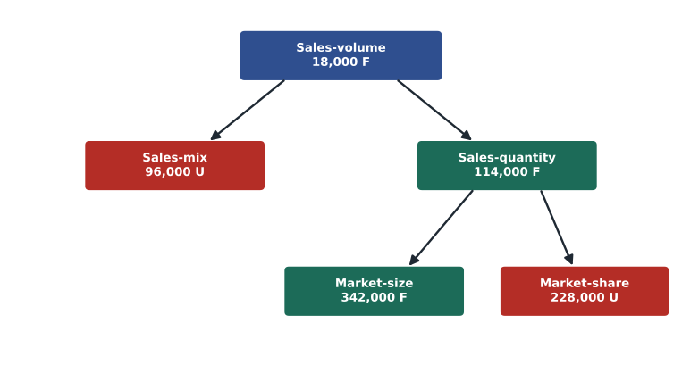
The analysis changes the story the headline tells. Halden sold more pumps than planned and the sales-volume variance is favorable, so a quick reading suggests a good year for sales. The deeper analysis shows that the market grew strongly, Halden failed to keep its share despite cutting the S-100's price, and the mix shifted toward the less profitable pump. The marketing team should be asked why commercial customers bought fewer P-300s, and whether competitors gained share with a new product. Market data must be reliable for this analysis; industry associations, trade data and syndicated research are common sources, and their definitions of the market must match the company's products.
Putting the sales and cost variances together
The selling-price variances net to $42,800 unfavorable. A complete reconciliation of budgeted to actual operating income for the year would start with the static-budget income, add the $18,000 favorable sales-volume variance to reach the flexible budget, then add the $42,800 unfavorable selling-price variance and the cost variances of lessons 8 and 9, such as the $53,000 of unfavorable machining overhead variances. Presented together, the variances tell a coherent story: Halden cut S-100 prices to fight for residential share, but the price cut did not hold share in a fast-growing market; commercial demand for the P-300 lagged; and the plant ran below its normal capacity, so fixed overhead was under-applied.
Reporting the cost of unused capacity
Lesson 9 showed that the choice of denominator level determines how much fixed overhead is labeled a production-volume variance. Many companies go one step further and report the cost of unused capacity explicitly. If Halden computed its machining fixed overhead rate on practical capacity of 22,000 machine hours, about $18.18 per hour, the fixed overhead not applied to products in a year of 18,500 standard hours would be about $63,600. Halden could then report that figure as a separate line, the cost of unused machining capacity, rather than burying it in product costs or in a variance account few managers read.
An explicit capacity cost line prompts better questions. Is the unused capacity temporary, because demand dipped, or permanent, because a product line has declined? Can it be sold, for example by taking contract machining work from other manufacturers at prices above variable cost? Should a machine be retired to cut fixed costs? Time-driven ABC in lesson 5 made the same point for support departments. Product costs computed on practical capacity tell sales staff what each pump really needs, while the capacity line tells executives what idle resources are costing them.
Inventory costing: absorption, variable and throughput
The second half of this lesson asks which manufacturing costs should be held in inventory until products are sold. Three approaches are used:
- Absorption costing includes all manufacturing costs in inventory: direct materials, direct labor, variable overhead and fixed overhead. It is required for external reporting.
- Variable (direct) costing includes only variable manufacturing costs in inventory and treats fixed manufacturing overhead as a period cost, expensed when incurred.
- Throughput (super-variable) costing includes only direct materials in inventory and treats all other manufacturing costs, including direct labor and variable overhead, as period costs. It reflects the view of the theory of constraints that, in the short run, only materials vary with output.
When production equals sales, all three give the same operating income. When production exceeds sales, absorption costing reports the highest income, because some fixed overhead is carried forward in inventory; throughput costing reports the lowest, because it expenses the most cost immediately. When sales exceed production, the order reverses.
# S-100 income under absorption, variable and throughput costing (illustrative)
price, produced, sold = 175, 21_000, 20_000
dm, dl, voh = 60, 32, 5            # variable manufacturing cost per pump
var_selling = 6
fixed_moh, normal_units = 600_000, 20_000
fixed_sa = 300_000

# Variable costing
var_cost = dm + dl + voh
vc_income = (price - var_cost - var_selling) * sold - fixed_moh - fixed_sa

# Absorption costing at normal capacity
fixed_rate = fixed_moh / normal_units
volume_var = fixed_moh - fixed_rate * produced        # negative = F
gross = (price - var_cost - fixed_rate) * sold - volume_var
ac_income = gross - var_selling * sold - fixed_sa

# Throughput costing
throughput = (price - dm) * sold
tc_income = throughput - (dl + voh) * produced - fixed_moh - var_selling * sold - fixed_sa

print(f"Variable costing income   {vc_income:>10,.0f}")
print(f"Absorption costing income {ac_income:>10,.0f}  (fixed OH in ending inventory "
      f"{(produced - sold) * fixed_rate:,.0f})")
print(f"Throughput costing income {tc_income:>10,.0f}  (DL and variable OH expensed on "
f"unsold pumps {(produced - sold) * (dl + voh):,.0f})")Variable costing income 540,000 Absorption costing income 570,000 (fixed OH in ending inventory 30,000) Throughput costing income 503,000 (DL and variable OH expensed on unsold pumps 37,000)
In the year shown, Halden produced 1,000 more S-100s than it sold. Absorption costing reports operating income of $570,000, because $30,000 of fixed overhead (1,000 pumps × $30) travels into ending inventory. Variable costing reports $540,000, because all $600,000 of fixed overhead is expensed. Throughput costing reports $503,000, because it also expenses the $37,000 of direct labor and variable overhead in the unsold pumps. The differences are purely about timing: over the life of the product, total income is the same under all three, because every cost is eventually expensed.
| Absorption | Variable | Throughput | |
|---|---|---|---|
| Costs in inventory | All manufacturing costs | Variable manufacturing costs | Direct materials only |
| S-100 inventory cost per pump | $127 | $97 | $60 |
| Operating income when production exceeds sales by 1,000 | $570,000 | $540,000 | $503,000 |
| Permitted for external reporting? | Yes (required) | No | No |
| Incentive to overproduce? | Yes | No | Negative (discourages it) |
Choosing a method for internal reporting
Because absorption costing rewards producing for inventory, many companies prepare internal reports on a variable or throughput basis, or combine absorption reports with controls on inventory levels. Variable costing aligns reported income with sales and makes the contribution margin visible, which supports the CVP and relevant-cost analyses of ACCT-102. Throughput costing goes further, strongly discouraging any production not matched to demand, which suits plants run with theory-of-constraints principles. Its weakness is that it treats direct labor as a fixed cost, which is realistic for many modern plants in the short run but less so for operations that adjust staffing with volume.
The choice of denominator level from lesson 9 interacts with the choice of method. Under absorption costing with a high denominator such as practical capacity, the fixed overhead rate is low, less fixed cost enters inventory, and the incentive to overproduce is weaker. Companies that want absorption-based reports without strong overproduction incentives sometimes combine practical-capacity rates with a policy of expensing the cost of unused capacity in the period.
External reporting and tax rules
For external reporting in the United States, ASC 330 requires absorption costing: inventory cost includes direct materials, direct labor and an allocation of fixed and variable production overhead based on normal capacity, while abnormal amounts of idle facility expense, freight, handling and spoilage are expensed. For federal income tax, the uniform capitalization rules of Internal Revenue Code section 263A (UNICAP) go further than GAAP: producers must capitalize not only direct costs but also an allocable share of indirect costs, including some costs that GAAP expenses, such as parts of purchasing, warehousing, and certain general and administrative costs, often using simplified methods. Small businesses whose average annual gross receipts over the prior three years do not exceed the inflation-adjusted threshold (about $32 million for tax years beginning in 2026) are exempt from UNICAP. Inventory measured at the lower of cost and net realizable value under GAAP (or lower of cost or market for LIFO and the retail method) cannot be written back up once written down.
Variable and throughput costing therefore remain internal tools. Companies that use them internally keep a reconciliation to absorption costing, adding the fixed overhead (and, for throughput, the other conversion costs) in beginning and ending inventory, so that internal and external figures can be tied together each period.
Common mistakes
MistakeComputing sales variances with revenue instead of contribution margin.
InsteadUse budgeted contribution margins so each variance measures its effect on operating income.
MistakeReading a favorable sales-volume variance as proof of strong sales performance.
InsteadSplit it into mix and quantity, and quantity into market size and share.
MistakeUsing the actual mix to compute the budgeted average contribution margin.
InsteadThe budgeted average CM uses the budgeted mix.
MistakeBelieving absorption costing income measures performance when inventory is building.
InsteadAbsorption income rises with overproduction; compare with variable costing or watch inventory levels.
MistakeUsing variable or throughput costing for external financial statements.
InsteadExternal reporting requires absorption costing; tax rules such as UNICAP may require even more costs in inventory.
Summary and key terms
- Sales variances use budgeted contribution margins to measure effects on operating income.
- The sales-volume variance splits into a sales-mix variance and a sales-quantity variance.
- The sales-quantity variance splits into market-size and market-share variances when market data are reliable.
- At Halden, an $18,000 favorable sales-volume variance hides a $96,000 unfavorable mix and a $228,000 unfavorable share loss in a growing market.
- Absorption costing includes all manufacturing costs in inventory; variable costing includes only variable manufacturing costs; throughput costing includes only materials.
- When production exceeds sales, absorption income is highest and throughput income lowest; over time the totals agree.
- External reporting requires absorption costing at normal capacity, and tax rules impose their own capitalization requirements.
- Uniform capitalization rules
- Tax rules under IRC section 263A requiring producers to capitalize direct and allocable indirect costs into inventory.
- Selling-price variance
- The difference between actual and budgeted price multiplied by actual units sold.
- Sales-volume variance
- The difference between actual and budgeted units multiplied by budgeted contribution margin.
- Sales-mix variance
- The effect on income of selling a different mix of products from budget.
- Sales-quantity variance
- The effect on income of selling a different total quantity from budget, at the budgeted mix.
- Market-size variance
- The effect on income of a difference between actual and budgeted market size.
- Market-share variance
- The effect on income of a difference between actual and budgeted market share.
- Absorption costing
- Inventory costing that includes all manufacturing costs.
- Variable costing
- Inventory costing that includes only variable manufacturing costs.
- Throughput costing
- Inventory costing that includes only direct materials.
- Budgeted average contribution margin
- Total budgeted contribution margin divided by total budgeted units at the budgeted mix.
Practice problems
Work each problem on paper first, then reveal the answer to check.
Budget: 10,000 units of A (CM $20) and 10,000 of B (CM $40). Actual: 12,000 A and 9,000 B. Compute the sales-volume variance.
Show answer
2,000 × 20 − 1,000 × 40 = $0.
For the same data, compute the sales-quantity variance.
Show answer
Average CM $30; (21,000 − 20,000) × 30 = $30,000 F.
Compute the sales-mix variance.
Show answer
$30,000 U, so that mix and quantity sum to zero.
Budgeted market 400,000 units at 5 percent; actual market 360,000 units; actual sales 21,000; average budgeted CM $30. Compute market-size and market-share variances.
Show answer
Size (−40,000) × 5% × 30 = $60,000 U; share (5.833% − 5%) × 360,000 × 30 = $90,000 F.
Halden's S-100 selling-price variance is $64,800 U. What decision does it reflect?
Show answer
A price cut of $3 per pump to win residential share.
If Halden produces 19,000 S-100s and sells 20,000 (with 1,000 in beginning inventory at $127), which method reports the highest income?
Show answer
Throughput costing, then variable, then absorption, because absorption releases fixed overhead from beginning inventory.
Reconcile variable and absorption income for the year shown in the lesson.
Show answer
Absorption $570,000 − variable $540,000 = $30,000 = 1,000 pumps × $30 fixed overhead in ending inventory.
Why might a plant manager prefer absorption-based bonuses?
Show answer
Producing extra units moves fixed overhead to inventory and raises reported income.
Name two costs excluded from inventory under IAS 2 or ASC 330.
Show answer
Abnormal waste and selling costs; also most storage and general administration.
How does UNICAP differ from GAAP inventory costing in the United States?
Show answer
It requires capitalizing additional indirect costs, such as parts of purchasing, warehousing and some administration, unless the small-business exemption applies.
Lesson quiz · 5 questions
Score 60% or more to complete this lesson.
Create a free account to save your progress, take quizzes and earn a certificate.