
ACCT-222 · Lesson 11 of 12 · 33 min
Cost estimation, learning curves and strategic cost management
Cost systems record what costs were; managers also need to predict what costs will be. This lesson begins with the quantitative tools for estimating cost behavior, extending the high–low and regression methods of ACCT-102 lesson 3 with a closer look at regression output and at learning curves, which capture the way labor time falls as workers gain experience. It then turns to strategic cost management: target costing and life-cycle costing, which manage costs before production begins; the cost of quality, which shows how spending on prevention can reduce total costs; lean accounting and backflush costing, which simplify the books in just-in-time plants; and a brief look at environmental and sustainability costing.
Estimating cost functions with regression
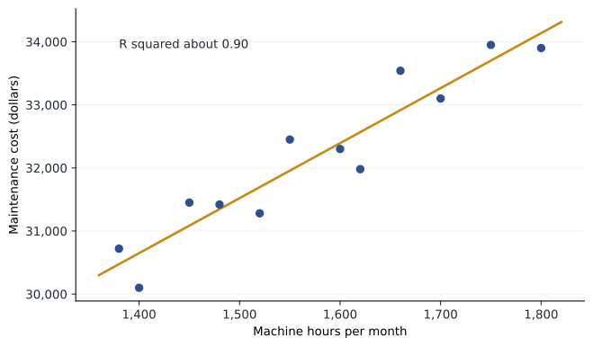
A cost function expresses a cost as a function of one or more cost drivers. The simplest form is linear: total cost = a + bX, where a is the fixed cost per period, b is the variable cost per unit of the driver and X is the quantity of the driver. Halden's plant maintenance department wants to estimate how its monthly cost varies with machine hours, both to budget and to check whether machine hours are a sensible allocation base. Twelve months of data are available.
| Month | Machine hours | Maintenance cost |
|---|---|---|
| Jan | 1,450 | $31,450 |
| Feb | 1,620 | $31,980 |
| Mar | 1,380 | $30,720 |
| Apr | 1,700 | $33,100 |
| May | 1,550 | $32,450 |
| Jun | 1,800 | $33,900 |
| Jul | 1,520 | $31,280 |
| Aug | 1,660 | $33,540 |
| Sep | 1,400 | $30,100 |
| Oct | 1,750 | $33,950 |
| Nov | 1,600 | $32,300 |
| Dec | 1,480 | $31,420 |
# Estimating the maintenance cost function: high-low versus least squares (illustrative)
from statistics import linear_regression, correlation, mean
mh = [1450, 1620, 1380, 1700, 1550, 1800, 1520, 1660, 1400, 1750, 1600, 1480]
cost = [31450, 31980, 30720, 33100, 32450, 33900, 31280, 33540, 30100, 33950, 32300, 31420]

# High-low uses only the highest and lowest activity months
hi, lo = mh.index(max(mh)), mh.index(min(mh))
b_hl = (cost[hi] - cost[lo]) / (mh[hi] - mh[lo])
a_hl = cost[hi] - b_hl * mh[hi]

# Least-squares regression uses every observation
b, a = linear_regression(mh, cost)
r2 = correlation(mh, cost) ** 2
pred = [a + b * x for x in mh]
resid = [y - p for y, p in zip(cost, pred)]
se = (sum(e * e for e in resid) / (len(mh) - 2)) ** 0.5
sxx = sum((x - mean(mh)) ** 2 for x in mh)
t_b = b / (se / sxx ** 0.5)

print(f"High-low:   cost = {a_hl:,.0f} + {b_hl:.2f} x MH")
print(f"Regression: cost = {a:,.0f} + {b:.2f} x MH")
print(f"R-squared {r2:.3f}; standard error of estimate {se:,.0f}; t for slope {t_b:.1f}")
print(f"Predicted cost at 1,700 MH: regression {a + b * 1700:,.0f}, high-low {a_hl + b_hl * 1700:,.0f}")High-low: cost = 20,271 + 7.57 x MH Regression: cost = 18,441 + 8.72 x MH R-squared 0.896; standard error of estimate 425; t for slope 9.3 Predicted cost at 1,700 MH: regression 33,265, high-low 33,143
The high–low method, which uses only the months with the highest and lowest machine hours, estimates a variable cost of about $7.57 per machine hour and fixed cost of about $20,271 a month. Least-squares regression, which uses all twelve months, estimates about $8.72 per machine hour and about $18,441 a month. The two methods disagree because the high and low months happen to contain random noise that the regression averages out. Regression is generally preferred for that reason.
Judging a regression
Three statistics help judge whether a regression is useful. The coefficient of determination (R²) measures the proportion of the variation in cost explained by the driver; here about 0.90, so machine hours explain about 90 percent of the month-to-month variation in maintenance cost. The standard error of the estimate, about $425, measures the typical size of the errors around the regression line, which helps managers set a realistic range around a budget. The t-statistic for the slope, about 9.3, measures whether the slope is reliably different from zero; values above about 2 suggest a genuine relationship.
Statistics are not enough on their own. A good cost function must also make economic sense: there should be a plausible reason why the driver causes the cost. Machine hours make sense for maintenance, because machines that run longer wear more. Managers should also check the data for problems before trusting any estimate: costs recorded in the wrong month, inflation over the period, a change in technology or methods, outliers caused by one-off events, and a relevant range that may not cover the activity level being forecast. When a cost depends on several drivers, such as machine hours and the number of set-ups, multiple regression can estimate the effect of each, provided the drivers are not too highly correlated with each other.
Learning curves
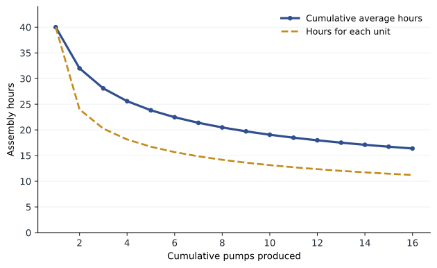
Many costs do not behave linearly because people and organizations learn. The first time Halden's technicians build a new custom pump design, they take a long time; by the eighth or sixteenth unit, they have learned the sequence, the jigs have been refined and the parts arrive in a more convenient order. A learning curve is a function that measures how labor hours per unit decline as cumulative output increases. The most common form, the cumulative average-time learning model, states that each time cumulative output doubles, the cumulative average time per unit falls to a constant percentage (the learning rate) of the previous average.
Here ȳ is the cumulative average time per unit, a is the time for the first unit, X is cumulative units produced, and b is the learning exponent. For an 80 percent learning rate, b = ln 0.8 ÷ ln 2 ≈ −0.3219. Halden is quoting on a new eight-pump order for the C-1200, a larger custom design based on the C-900. Engineering estimates 40 direct labor hours for the first pump and an 80 percent learning rate.
# Cumulative average-time learning curve, 80% (illustrative)
from math import log
first, rate = 40.0, 0.80
b = log(rate) / log(2)
print(f"Learning exponent b = {b:.4f}")
print(f"{'Units':>5} {'Cum. avg hrs':>13} {'Total hrs':>10} {'Hrs for last unit':>18}")
prev_total = 0
for x in (1, 2, 4, 8, 16):
    avg = first * x ** b
    total = avg * x
    last = total - ((x - 1) * first * (x - 1) ** b if x > 1 else 0)
    print(f"{x:>5} {avg:>13.2f} {total:>10.2f} {last:>18.2f}")
wage, oh_per_hr = 36, 50
hrs8 = first * 8 ** b * 8
print(f"Wages and hour-driven overhead for 8 pumps: {hrs8:.1f} h x ${wage + oh_per_hr} "
f"= ${hrs8 * (wage + oh_per_hr):,.0f}; ignoring learning: ${8 * first * (wage + oh_per_hr):,.0f}")Learning exponent b = -0.3219
Units Cum. avg hrs Total hrs Hrs for last unit
1 40.00 40.00 40.00
2 32.00 64.00 24.00
4 25.60 102.40 18.15
8 20.48 163.84 14.18
16 16.38 262.14 11.22
Wages and hour-driven overhead for 8 pumps: 163.8 h x $86 = $14,090; ignoring learning: $27,520With 80 percent learning, the cumulative average falls from 40 hours for the first pump to 32 for the first two, 25.6 for four and 20.48 for eight. Eight pumps take about 164 hours in total rather than the 320 hours a naive estimate would give. At an illustrative $36 an hour of wages and $50 an hour of labor-driven overhead, ignoring learning would overstate the cost of the order by about $13,400 and could lose the bid. Conversely, using the eight-unit average to price the very first pump of a one-off order would understate its cost.
Learning curves matter in bidding, in setting standards for new products (a standard based on mature output will produce large unfavorable variances in the early months), in budgeting and in make-or-buy decisions. The learning rate itself must be estimated from experience on similar products; rates between 70 and 90 percent are common in assembly work, with lower rates (faster learning) for complex manual tasks and higher rates for highly automated processes. An alternative, the incremental unit-time model, applies the learning rate to the time for each additional unit rather than to the cumulative average and gives somewhat higher total times for the same rate.
Target costing
Most of a product's cost is committed at the design stage, long before production starts. Once the parts, materials, tolerances and manufacturing process are chosen, the plant can only manage costs at the margin. Target costing works backward from the market: it starts with the price customers will pay, subtracts the margin the company needs, and treats the result as the maximum cost the product may have. Engineers, purchasing and production then use value engineering to design a product that meets the target.
Worked problem
Target costing a compact residential pump
Halden's marketing team believes a new compact pump, the S-50, can sell to dealers at $140 against competing imports. Halden requires a 20 percent margin on price to cover selling, service and profit. Engineering's first design has an estimated full manufacturing cost of $128. What is the cost gap, and how might it be closed?
Show solution
- Target margin = 20% × $140 = $28; target cost = $140 − $28 = $112.
- Cost gap = $128 − $112 = $16 per pump.
- Value engineering ideas: use the S-100 motor and seal kit rather than new parts (saving set-up, engineering and purchasing costs per lesson 4); replace a two-piece cast housing with a one-piece molded housing from Grade A recovered resin (lesson 7); reduce fasteners from 14 to 8.
- Engineering estimates these changes cut cost to $110, below the target.
Answer: The target cost is $112; value engineering closes the $16 gap before production starts.
Target costing is most valuable in competitive markets where prices are set by competitors and customers rather than by cost-plus formulas. It depends on cross-functional teams, accurate cost estimates at the design stage (ABC data are especially useful here, because they show the cost of complexity) and discipline: if the target cannot be met, the product should not be launched. Many Japanese and North American automotive and electronics companies use target costing routinely.
Life-cycle costing
Life-cycle costing tracks all the costs of a product from its initial research and development through design, production, marketing, distribution and customer service, until it is withdrawn. Because external financial reports show research, development, marketing and service costs as period expenses in the years they occur, they never show whether a product was profitable over its whole life. A life-cycle budget does.
# Life-cycle budget for the S-50 compact pump (illustrative, in thousands of dollars)
years = ["Y1", "Y2", "Y3", "Y4", "Y5", "Y6"]
units = [0, 4, 12, 16, 14, 8]                     # thousands of pumps
price, unit_cost = 140, 110                       # dollars per pump
rnd_design = [450, 150, 0, 0, 0, 0]
marketing = [60, 220, 150, 120, 90, 40]
service_per_unit = 6                              # warranty and support, dollars
total = 0
for y, u, r, m in zip(years, units, rnd_design, marketing):
    contribution = u * (price - unit_cost - service_per_unit)
    profit = contribution - r - m
    total += profit
    print(f"{y}: units {u:>3}k  contribution {contribution:>5,.0f}  R&D/design {r:>4}  "
f"marketing {m:>4} profit {profit:>6,.0f} cumulative {total:>6,.0f}")Y1: units 0k contribution 0 R&D/design 450 marketing 60 profit -510 cumulative -510 Y2: units 4k contribution 96 R&D/design 150 marketing 220 profit -274 cumulative -784 Y3: units 12k contribution 288 R&D/design 0 marketing 150 profit 138 cumulative -646 Y4: units 16k contribution 384 R&D/design 0 marketing 120 profit 264 cumulative -382 Y5: units 14k contribution 336 R&D/design 0 marketing 90 profit 246 cumulative -136 Y6: units 8k contribution 192 R&D/design 0 marketing 40 profit 152 cumulative 16
The life-cycle budget shows the S-50 losing money in its first two years, as development, design and launch marketing outweigh early sales. The product only recovers its development and launch costs in its final year, with a cumulative profit of about $16,000 over six years. Annual income statements would show healthy profits in years 3 to 6 and hide how thin the product's overall return really is. A discounted cash-flow analysis, as in FIN-201, would refine the figure by recognizing the time value of money. The budget also highlights the importance of the early stages: a $100,000 design change that cuts service costs by $2 per pump over 54,000 pumps would add about $8,000 of life-cycle profit before discounting, which would raise the S-50's thin life-cycle profit by half. These are the trade-offs target costing and life-cycle costing make visible.
The cost of quality
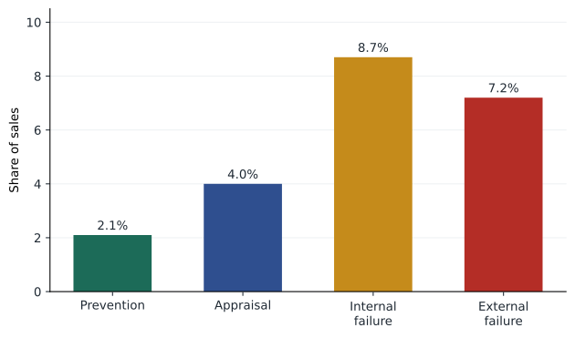
The cost of quality (COQ) groups the costs incurred to prevent or remedy poor quality into four categories. Prevention costs are incurred to stop defects from happening: design reviews, supplier evaluation, training, process engineering. Appraisal costs detect defects before products reach customers: incoming inspection, pressure testing, quality audits. Internal failure costs arise from defects caught before shipment: spoilage, rework, scrap and the downtime they cause. External failure costs arise from defects found by customers: warranty repairs, returns, product liability, and the lost sales from damaged reputation, often the largest and least visible cost.
# Halden cost of quality report for the year (illustrative, dollars)
sales = 20_000 * 175 + 5_000 * 390 + 500 * 1_650
coq = {
    "Prevention": {"Design reviews": 60_000, "Supplier evaluation": 30_000, "Training": 40_000},
    "Appraisal": {"Pressure testing and inspection": 200_000, "Incoming materials inspection": 50_000},
    "Internal failure": {"Spoilage": 420_000, "Rework": 80_000, "Downtime from defects": 45_000},
    "External failure": {"Warranty repairs (Halden Service)": 380_000, "Returns and freight": 70_000},
}
total = 0
for cat, items in coq.items():
    sub = sum(items.values())
    total += sub
    print(f"{cat:<17} {sub:>9,}  {sub / sales:5.1%} of sales")
print(f"{'Total':<17} {total:>9,} {total / sales:5.1%} of sales (sales ${sales:,})")Prevention 130,000 2.1% of sales Appraisal 250,000 4.0% of sales Internal failure 545,000 8.7% of sales External failure 450,000 7.2% of sales Total 1,375,000 21.9% of sales (sales $6,275,000)
Halden's measured quality costs total $1,375,000, about 21.9 percent of sales of $6,275,000, and they exclude the hardest cost to measure, sales lost because dealers lost confidence. Prevention is only 2.1 percent of sales, while failure costs (internal and external) are about 15.9 percent. The classic lesson of the cost of quality is that this pattern is backward: a dollar spent on prevention typically saves several dollars of appraisal and failure cost. Halden's seal failures, which drive much of its spoilage and warranty cost, could be attacked with a supplier quality program and a redesigned seal seat, both prevention costs. Quality costs reported this way also tie together earlier lessons: spoilage and rework from lesson 3, inspection activity costs from lesson 4 and warranty claims handled in lesson 5.
Lean accounting and backflush costing
Plants that adopt just-in-time production and lean methods hold little inventory, make products in small batches pulled by customer demand, and organize work in cells or value streams rather than functional departments. In such plants, tracking every cost through work in process with detailed job sheets or production reports adds cost without adding much information. Lean accounting simplifies: it organizes costs by value stream (all the steps that make a product family), reports value-stream profit and a small set of operational measures, and uses simplified inventory costing.
Backflush costing is the main simplified method. Instead of recording each movement of materials and labor, it waits until a trigger point, such as the completion or sale of finished units, and then works backward ('flushes' costs back) to record the standard cost of the units produced or sold. Work in process may not be recorded at all. Conversion costs are often combined into one account, recognizing that direct labor is a small and fixed element in automated cells.
Worked problem
Backflush costing for an S-100 cell
Halden runs a lean cell for S-100 final assembly with standard materials of $112 and standard conversion of $45 per pump. In March it bought $2,250,000 of materials, incurred $910,000 of conversion costs, completed 20,000 pumps and sold 19,800. Trigger points are the purchase of materials and the completion of finished goods. Record the main entries.
Show solution
- Purchase: debit Materials and in-process inventory $2,250,000; credit Accounts payable $2,250,000.
- Conversion costs incurred: debit Conversion costs control $910,000; credit various accounts $910,000.
- Completion (trigger point): debit Finished goods 20,000 × $157 = $3,140,000; credit Materials and in-process inventory $2,240,000 and Conversion costs allocated $900,000.
- Sale: debit Cost of goods sold 19,800 × $157 = $3,108,600; credit Finished goods $3,108,600.
- Under-allocated conversion of $10,000 ($910,000 − $900,000) is written off to cost of goods sold at period-end.
Answer: Two inventory accounts and a handful of entries replace detailed work-in-process tracking.
Backflush costing works when inventories are low and stable and standard costs are accurate; otherwise it can misstate inventory and hide losses that a detailed system would catch. It is acceptable for external reporting only if the results approximate those of conventional absorption costing, which is usually the case when inventories are small.
Environmental and sustainability costing
Environmental costs, such as waste disposal, emissions permits, effluent treatment, energy and compliance staff, are often buried in general overhead and allocated with volume-based rates, so products that create the most environmental cost are not charged for it. Activity-based approaches can trace these costs to the products and processes that cause them. Material flow cost accounting, described in ISO 14051, tracks the flows of materials and energy through a process and values the material that leaves as waste at its full cost of materials, energy and processing, which is often much larger than the disposal fee alone. Halden's resin recovery line from lesson 7 is partly a response to such an analysis: scrapped housings that were once sent to landfill at a disposal fee are now a source of Grade A resin. Carbon pricing and climate disclosure requirements are increasing the demand for product-level emissions data, which raises the same allocation questions that cost accountants have long faced with joint and shared costs.
Common mistakes
MistakeTrusting the high-low method because it is simple.
InsteadPrefer regression, which uses all the data, and check R², the standard error and the slope's t-statistic.
MistakeAccepting a regression with a high R² but no economic logic.
InsteadRequire a plausible cause-and-effect link between driver and cost.
MistakePricing a long production run at the first-unit cost.
InsteadApply the learning curve to estimate cumulative hours for the whole order.
MistakeSetting the target cost from current costs plus a markup.
InsteadStart from the market price and the required margin; then engineer the product to meet the target.
MistakeCutting prevention spending to reduce quality costs.
InsteadPrevention usually reduces appraisal and failure costs by more than it costs.
Summary and key terms
- Cost functions estimate fixed and variable components; regression is preferred to the high-low method.
- R², the standard error of the estimate and the slope t-statistic help judge a regression, alongside economic plausibility and data checks.
- Under a cumulative average-time learning curve, the average time per unit falls to the learning rate each time cumulative output doubles.
- Target costing works back from market price and required margin, using value engineering to meet the target.
- Life-cycle costing tracks all costs over a product's life, revealing whether it is profitable overall.
- The cost of quality groups prevention, appraisal, internal failure and external failure costs; prevention usually pays for itself.
- Lean accounting and backflush costing simplify the books in low-inventory plants; environmental costing traces hidden environmental costs to their causes.
- Cost function
- A mathematical description of how a cost changes with a cost driver.
- Coefficient of determination
- The proportion of variation in the dependent variable explained by the regression (R²).
- Standard error of the estimate
- A measure of the typical deviation of actual values from the regression line.
- Learning curve
- A function showing how labor time per unit declines as cumulative output increases.
- Cumulative average-time learning model
- A learning model in which the cumulative average time per unit falls by a constant rate when output doubles.
- Target cost
- Target price minus target margin; the maximum allowable cost of a product.
- Value engineering
- Systematic evaluation of product design to reduce cost while meeting customer needs.
- Life-cycle costing
- Tracking and accumulating costs over a product's entire life.
- Cost of quality
- Costs of preventing, detecting and remedying poor quality.
- Backflush costing
- A simplified system that records costs at trigger points and works backward to assign standard costs.
Practice problems
Work each problem on paper first, then reveal the answer to check.
Using the regression, predict maintenance cost at 1,500 machine hours.
Show answer
About 18,441 + 8.72 × 1,500 ≈ $31,520.
Why might the high-low estimate differ from the regression estimate?
Show answer
High-low uses only two months, which may contain unusual noise; regression uses all data.
An R² of 0.20 is reported for a cost and a proposed driver. What should managers conclude?
Show answer
The driver explains little of the variation; look for a better driver or additional drivers.
With a 90 percent cumulative average-time curve and 50 hours for the first unit, what is the cumulative average for four units?
Show answer
50 × 0.9 × 0.9 = 40.5 hours.
What is the total time for those four units?
Show answer
162 hours.
A product's target price is $80 and the target margin is 25 percent of price. What is the target cost?
Show answer
$60.
Classify: pressure testing, warranty repair, supplier audits, remelting cracked castings.
Show answer
Appraisal; external failure; prevention; internal failure.
Halden adds $50,000 of seal design work. Failure costs fall by $180,000. What is the net effect on quality costs?
Show answer
A net reduction of $130,000.
Under backflush costing with a sale trigger only, what account is debited when units are sold?
Show answer
Cost of goods sold at standard cost, with credits to materials and conversion accounts.
Why does material flow cost accounting often show waste costs much larger than disposal fees?
Show answer
It values waste at the full cost of materials, energy and processing embedded in it.
Lesson quiz · 5 questions
Score 60% or more to complete this lesson.
Create a free account to save your progress, take quizzes and earn a certificate.