The upper atmosphere and the ionosphere: photoionization and layers

Above about 60 km the Sun's most energetic photons, in the extreme ultraviolet and X-ray ranges, have not yet been absorbed, and they carry enough energy to knock electrons out of atoms and molecules. The freed electrons and the positive ions they leave behind form the ionosphere, a weakly ionized plasma that coexists with the much denser neutral gas. Its electron density rises from almost nothing at 60 km to a peak of about \(10^{12}\) per cubic metre near 300 km by day, then falls slowly toward the magnetosphere. The ionosphere is not a single layer but several, labelled D, E, F1 and F2, and its structure changes with the time of day, the season, the solar cycle and geomagnetic storms. This lesson explains where the layers come from, using Sydney Chapman's 1931 theory of photoionization in an exponential atmosphere, the balance between production and loss, and the photochemistry that distinguishes one layer from the next.

Photoionization

A photon ionizes an atom or molecule if its energy exceeds the ionization energy. The program below converts the ionization energies of the main upper-atmosphere species into threshold wavelengths. Molecular nitrogen, with an ionization energy of 15.6 eV, needs photons shorter than about 80 nm; atomic oxygen needs shorter than 91 nm; molecular oxygen, 103 nm. Nitric oxide, a minor species with an ionization energy of only 9.3 eV, can be ionized by the strong hydrogen Lyman-alpha line of the Sun at 121.6 nm, which penetrates deeper because the major gases do not absorb it strongly. Each wavelength band is absorbed at a different height, depending on the cross-section of the gases that absorb it, and that is the origin of the layers.

The solar spectrum at these wavelengths is variable. The extreme ultraviolet flux changes by a factor of two or more over the 11-year solar cycle, and the X-ray flux by a factor of ten or more, with much larger and faster increases during flares. The ionosphere follows these changes: near solar maximum, as in 2024 and 2025, the F2 layer is denser and higher, and the thermosphere hotter and more extended, than near solar minimum.

Chapman's production function

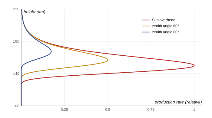
Consider monochromatic radiation of intensity \(I_\infty\) arriving at the top of an isothermal atmosphere at a solar zenith angle \(\chi\), the angle between the Sun and the vertical. The absorbing gas has number density \(n(z) = n_0 e^{-z/H}\) and absorption cross-section \(\sigma\). The optical depth above height \(z\) along the slanted path is \(\tau = \sigma n(z) H\sec\chi\), and each absorbed photon produces an ion pair with efficiency \(\eta\). The production rate per unit volume is the absorption rate,

The production is a competition: high up, there is plenty of radiation but little gas to absorb it; low down, there is plenty of gas but the radiation has already been used up. The maximum occurs where \(dq/dz = 0\), which gives \(\tau = 1\): the production peaks where the optical depth along the path is one. With the reduced height \(y = (z - z_{m0})/H\), measured from the height \(z_{m0}\) of the peak for an overhead Sun, Chapman's function takes the universal form

As the Sun moves away from the zenith, the peak rises by \(H\ln\sec\chi\) and its rate falls in proportion to \(\cos\chi\). The program checks these results numerically.

import math
# Chapman production function: q(z) = q_m0 exp(1 - y - sec(chi) exp(-y)), y = (z - z_m0)/H
H = 10.0; z_m0 = 150.0; q_m0 = 1.0
def q(z, chi):
    y = (z - z_m0) / H
    return q_m0 * math.exp(1 - y - math.exp(-y) / math.cos(math.radians(chi)))
print(" chi (deg)   peak height (km)   peak rate (relative)   predicted peak")
for chi in (0, 30, 60, 75, 85):
    zs = [z_m0 - 60 + 0.01 * i for i in range(14001)]
    zp = max(zs, key=lambda z: q(z, chi))
    sec = 1 / math.cos(math.radians(chi))
    print(f"   {chi:4d}       {zp:8.2f}           {q(zp, chi):8.4f}        z = {z_m0 + H * math.log(sec):.2f}, q = {math.cos(math.radians(chi)):.4f}")

# Photon energies and the ionization thresholds that set which wavelengths ionize which gas
h = 6.62607015e-34; c = 2.99792458e8; eV = 1.602176634e-19
for gas, E in [("NO", 9.26), ("O2", 12.07), ("O", 13.62), ("H", 13.60), ("N2", 15.58), ("He", 24.59)]:
    print(f"{gas:3s} ionization energy {E:5.2f} eV -> photons shorter than {h * c / (E * eV) * 1e9:6.1f} nm")
print(f"hydrogen Lyman-alpha 121.6 nm carries {h * c / 121.6e-9 / eV:.2f} eV: it ionizes NO but not O2")

# Equilibrium electron density in an E-region layer with recombination alpha: n = sqrt(q/alpha)
alpha = 3e-13   # m^3/s, dissociative recombination
for qq in (1e9, 3e9, 1e10):
    print(f"production {qq:.0e} per m^3 per s -> electron density {math.sqrt(qq / alpha):.2e} per m^3")
# After sunset: n(t) = n0 / (1 + alpha n0 t)
n0 = math.sqrt(3e9 / alpha)
for t in (60, 600, 3600):
    print(f"  {t:5d} s after production stops: {n0 / (1 + alpha * n0 * t):.2e} per m^3")

 chi (deg)   peak height (km)   peak rate (relative)   predicted peak
      0         150.00             1.0000        z = 150.00, q = 1.0000
     30         151.44             0.8660        z = 151.44, q = 0.8660
     60         156.93             0.5000        z = 156.93, q = 0.5000
     75         163.52             0.2588        z = 163.52, q = 0.2588
     85         174.40             0.0872        z = 174.40, q = 0.0872
NO  ionization energy  9.26 eV -> photons shorter than  133.9 nm
O2  ionization energy 12.07 eV -> photons shorter than  102.7 nm
O   ionization energy 13.62 eV -> photons shorter than   91.0 nm
H   ionization energy 13.60 eV -> photons shorter than   91.2 nm
N2  ionization energy 15.58 eV -> photons shorter than   79.6 nm
He  ionization energy 24.59 eV -> photons shorter than   50.4 nm
hydrogen Lyman-alpha 121.6 nm carries 10.20 eV: it ionizes NO but not O2
production 1e+09 per m^3 per s -> electron density 5.77e+10 per m^3
production 3e+09 per m^3 per s -> electron density 1.00e+11 per m^3
production 1e+10 per m^3 per s -> electron density 1.83e+11 per m^3
     60 s after production stops: 3.57e+10 per m^3
    600 s after production stops: 5.26e+09 per m^3
   3600 s after production stops: 9.17e+08 per m^3

The numerical peaks agree with the analytic predictions to the printed precision: for a scale height of 10 km, the peak at a zenith angle of 60° is 6.9 km higher and half as strong as for an overhead Sun, and at 85° it is 24 km higher and less than a tenth as strong. The theory explains why the ionosphere is weakest and highest near sunrise and sunset, and why in winter at high latitudes, where the Sun stays low, the lower layers almost disappear.

Loss: recombination and attachment

Electrons are removed by recombination with positive ions. For molecular ions such as \(\mathrm{O_2^+}\) and \(\mathrm{NO^+}\), dissociative recombination, \(\mathrm{NO^+} + e \to \mathrm{N} + \mathrm{O}\), is fast, with a rate coefficient \(\alpha \approx 3\times10^{-13}\) m\(^3\)/s. Because loss requires an electron and an ion to meet, the loss rate is \(\alpha n_e n_i = \alpha n_e^2\), and in equilibrium with production \(q\),

This is the Chapman layer: its electron density follows the square root of the production profile. After sunset, with production switched off, \(dn_e/dt = -\alpha n_e^2\) gives \(n_e(t) = n_0/(1 + \alpha n_0 t)\), a decay that is fast at first and then slows. In the program, an E-region density of \(10^{11}\) per m\(^3\) falls by a factor of about three in a minute and by a factor of a hundred in an hour. That is why the E layer nearly vanishes at night, leaving only a weak residue maintained by starlight, scattered Lyman radiation and meteors.

In the F region the main ion is atomic \(\mathrm{O^+}\), which cannot recombine dissociatively. Its radiative recombination is extremely slow, so loss goes in two steps: \(\mathrm{O^+}\) first exchanges its charge with \(\mathrm{N_2}\) or \(\mathrm{O_2}\) to form a molecular ion, which then recombines quickly. The first step depends on the density of molecular nitrogen and oxygen, which falls with height faster than atomic oxygen does. The loss rate therefore decreases with height faster than the production rate, and the electron density keeps rising above the production peak. The F2 peak, near 250 to 350 km, forms where this chemical loss gives way to diffusion along magnetic field lines, which carries plasma downward. Because loss is slow at these heights, the F2 layer survives the night, which is what makes long-distance shortwave radio possible after dark.

The layers

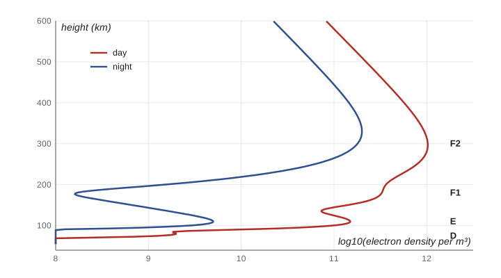
The D region, from about 60 to 90 km, is formed by Lyman-alpha ionizing nitric oxide and by hard X-rays and cosmic rays ionizing everything. Its densities are only about \(10^8\) to \(10^9\) per m\(^3\), but the neutral gas is dense, so electrons collide frequently and absorb energy from radio waves passing through. The D region is why AM radio stations are heard only locally by day and far away at night: the daytime D region absorbs their signals before they reach the reflecting layers above. It disappears at night. During a strong solar X-ray flare, its ionization rises suddenly and shortwave signals on the sunlit side of the Earth fade within minutes, a radio blackout.

The E region, from about 90 to 150 km, peaks near 110 km at about \(10^{11}\) per m\(^3\), formed by soft X-rays and extreme ultraviolet ionizing molecular oxygen and nitrogen. It is the closest of the layers to an ideal Chapman layer, varying smoothly with the Sun's zenith angle. In summer, thin, dense patches called sporadic E form at about 100 to 110 km from metal ions deposited by meteors and concentrated by wind shear; they can reflect even television and FM signals over 1000 to 2000 km for an hour or two.

The F1 layer, a ledge near 180 km, appears only by day and is most pronounced in summer and at solar minimum. Above it, the F2 layer is the densest part of the ionosphere and the most variable. It does not behave like a Chapman layer: its peak density is often larger in winter than in summer at mid-latitudes, a puzzle called the winter anomaly, which comes from seasonal changes in the composition of the neutral gas. Near the magnetic equator, the F2 layer forms two crests about 15° on either side, because daytime electric fields lift plasma upward, and it then slides down the magnetic field lines to higher latitudes. At high latitudes the F2 layer is shaped by the convection of plasma across the polar cap and by particle precipitation in the auroral zone, which lessons 10 and 11 describe.

Ionospheric currents

The ionosphere conducts electricity, and in the E region, between about 90 and 150 km, it conducts it in an unusual way. Below about 100 km, electrons collide so often with neutral molecules that they cannot circle around magnetic field lines, while above about 130 km ions as well as electrons gyrate freely. In between, electrons gyrate but ions are dragged along by the neutral wind, and the two species respond to electric fields differently. The result is a conductivity that depends on direction: high along the magnetic field, lower across it, and with a Hall component at right angles to both the field and the electric field. Tidal winds driven by solar heating push the conducting E region across the Earth's magnetic field, generating a dynamo current system on the dayside, called the Sq current, that produces daily magnetic variations of a few tens of nanotesla at the ground. Carl Friedrich Gauss and Balfour Stewart, in the nineteenth century, inferred from these variations that a conducting layer must exist high above the Earth, long before radio confirmed it. In the auroral zone, electrojet currents of a million amperes flow during substorms and produce ground disturbances of a thousand nanotesla or more, the ultimate source of the induced currents in power grids discussed in lesson 12.

Measuring the ionosphere

The ionosonde, developed from the experiments of Edward Appleton in England and of Gregory Breit and Merle Tuve in the United States in the mid-1920s, sweeps a radio transmitter from about 1 to 20 MHz and times the echoes from directly overhead. Each frequency reflects from the height where it equals the local plasma frequency, so the record, an ionogram, maps electron density up to the peak. Lesson 8 develops this. Incoherent scatter radars, such as those at Millstone Hill in Massachusetts and at Poker Flat in Alaska, detect the faint scattering of powerful radar pulses by individual electrons, giving density, temperature and velocity at all heights. Satellites sound the ionosphere from above, as Canada's Alouette 1 did from 1962, and today the delay of GNSS signals on their way to thousands of ground receivers gives continuous global maps of total electron content.