Capstone: space weather — impacts on power grids, satellites, aviation and forecasting

At 2:44 in the morning on 13 March 1989, a surge of the geomagnetic field over Québec tripped protective relays on the Hydro-Québec transmission network. Within 92 seconds the grid that carried power from the James Bay hydroelectric stations to the south had collapsed, and about six million people were without electricity, many of them for about nine hours in winter. The same storm damaged a large transformer at the Salem nuclear plant in New Jersey and caused navigation problems for satellites. Space weather is the practical end of this course: the chain from the Sun to the ground that the previous lessons built, applied to the systems modern society depends on. This capstone follows that chain into power grids, satellites, navigation and communications, aviation and human spaceflight, and then describes how space weather is observed and forecast, and how utilities and operators prepare.

The chain of cause and effect

A space weather event usually begins with a solar eruption. A flare's X-rays reach the Earth in eight minutes and cause shortwave radio blackouts on the day side (lesson 8). Solar energetic particles, protons accelerated by the flare and by the shock ahead of a coronal mass ejection, arrive within tens of minutes to hours, travel along the Parker spiral (lesson 9) and pour into the polar caps, causing polar cap absorption and radiation hazards. The ejection itself arrives one to four days later. If its magnetic field points south, it drives reconnection, the ring current grows, substorms intensify, and the auroral oval expands (lessons 10 and 11). Currents of millions of amperes flow in the ionosphere, and their rapidly changing magnetic fields at the ground induce electric fields in the conducting Earth. Meanwhile the energy dissipated in the upper atmosphere heats and expands the thermosphere, increasing the drag on low satellites. Each link has its own effect on technology, and NOAA rates them on three five-level scales: R for radio blackouts, S for solar radiation storms and G for geomagnetic storms.

Geomagnetically induced currents

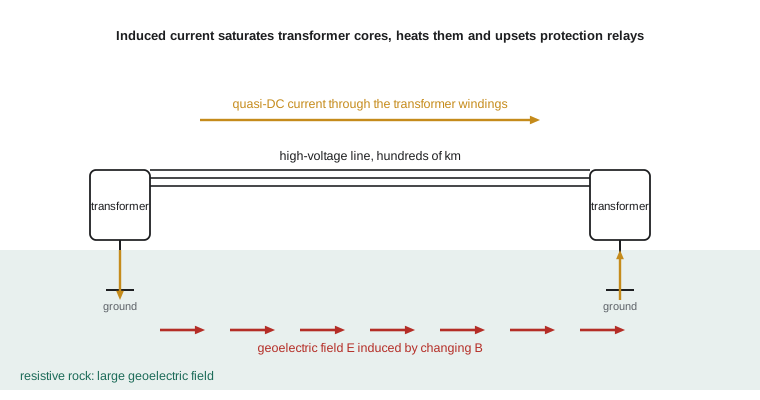
By Faraday's law, a magnetic field that changes in time induces an electric field. When the field at the ground changes during a storm, the electric field drives currents in the conducting Earth, and where a transmission line is grounded at both ends, the line offers a low-resistance path in parallel with the ground. A quasi-DC current, varying over minutes, then flows into the grid through the neutral connections of transformers. Transformers are designed for alternating current; a DC offset of a few tens of amperes pushes their iron cores into saturation for half of each cycle. Saturated transformers draw large distorted currents rich in harmonics, consume reactive power, overheat locally and can trip protective relays designed for normal faults. In 1989 it was the relays on static VAR compensators, devices that stabilize the voltage on long lines, that tripped first and brought down the Hydro-Québec grid.

The size of the geoelectric field depends on how fast the magnetic field changes and on the conductivity of the ground. PHYS-382 showed that a wave of angular frequency \(\omega\) penetrates a conductor of conductivity \(\sigma\) to a skin depth \(\delta = \sqrt{2/\omega\mu_0\sigma}\). For a uniform conducting half-space, the ratio of surface electric field to magnetic field, the surface impedance, gives

The program below applies this to a disturbance of 500 nT per minute with a 5-minute period, typical of a strong storm at high latitude. Over resistive igneous rock with \(\sigma = 10^{-4}\) S/m, the field is about 5 V/km; over conductive sediments it is thirty times smaller. The Canadian Shield, which underlies much of Québec, Ontario and Manitoba, is exactly such resistive rock, which is one reason Hydro-Québec was so vulnerable. The program then estimates the current in a grounded line, compares satellite drag at 210 km in quiet and storm conditions, computes the warning time from a monitor at L1, and gives illustrative radiation doses on a long polar flight.

import math
mu0 = 4e-7 * math.pi
# Geoelectric field from a magnetic disturbance over a uniform conducting Earth: |E| = |B| sqrt(omega / (mu0 sigma))
dBdt = 500e-9 / 60          # 500 nT per minute
period = 300.0              # dominant period of the disturbance (s)
w = 2 * math.pi / period
B = dBdt / w
print(f"500 nT/min at a {period:.0f} s period: amplitude {B * 1e9:.0f} nT")
for ground, sig in [("resistive shield rock", 1e-4), ("average ground", 1e-3), ("conductive sediments", 1e-1)]:
    E = B * math.sqrt(w / (mu0 * sig))
    depth = math.sqrt(2 / (w * mu0 * sig))
    print(f"  {ground:22s} sigma {sig:.0e} S/m: E = {E * 1000:6.2f} V/km, skin depth {depth / 1000:5.0f} km")

# Quasi-DC current in a grounded transmission line: I = E L / (R_line + 2 R_ground + R_transformers)
E = B * math.sqrt(w / (mu0 * 1e-4))
for Lkm in (100, 300, 700):
    R_line = 0.03 * Lkm; R_rest = 2 * 0.5 + 2 * 0.3
    I = E * Lkm * 1000 / (R_line + R_rest)
    print(f"line {Lkm:3d} km: driving voltage {E * Lkm * 1000:6.0f} V, induced current {I:5.0f} A (about {I / 3:.0f} A per phase)")

# Satellite drag: storm heating raises thermospheric density; decay rate da/dt = -sqrt(G M a) rho Cd A / m
GM = 3.986e14; RE = 6.371e6
a = RE + 210e3; Cd, A, m = 2.2, 4.0, 260.0
for label, rho in [("quiet", 2.0e-10), ("storm", 5.0e-10)]:
    dadt = -math.sqrt(GM * a) * rho * Cd * A / m
    print(f"{label:5s} density {rho:.1e} kg/m^3 at 210 km: orbit decays {-dadt * 86400 / 1000:.1f} km per day")

# Alert lead times from a monitor at L1, 1.5 million km upstream
L1 = 1.5e9
for v in (400e3, 800e3, 2000e3):
    print(f"solar wind at {v / 1e3:.0f} km/s crosses L1 to Earth in {L1 / v / 60:.0f} min")

# Radiation dose on a long polar flight (illustrative rates, microsievert per hour)
for label, rate, hours in [("quiet sun, polar route", 5.0, 10), ("strong solar particle event", 20.0, 10), ("sea level background", 0.1, 10)]:
    print(f"{label:28s} {rate * hours:6.1f} uSv over {hours} h")

500 nT/min at a 300 s period: amplitude 398 nT
  resistive shield rock  sigma 1e-04 S/m: E =   5.14 V/km, skin depth   872 km
  average ground         sigma 1e-03 S/m: E =   1.62 V/km, skin depth   276 km
  conductive sediments   sigma 1e-01 S/m: E =   0.16 V/km, skin depth    28 km
line 100 km: driving voltage    514 V, induced current   112 A (about 37 A per phase)
line 300 km: driving voltage   1541 V, induced current   145 A (about 48 A per phase)
line 700 km: driving voltage   3596 V, induced current   159 A (about 53 A per phase)
quiet density 2.0e-10 kg/m^3 at 210 km: orbit decays 30.0 km per day
storm density 5.0e-10 kg/m^3 at 210 km: orbit decays 74.9 km per day
solar wind at 400 km/s crosses L1 to Earth in 62 min
solar wind at 800 km/s crosses L1 to Earth in 31 min
solar wind at 2000 km/s crosses L1 to Earth in 12 min
quiet sun, polar route         50.0 uSv over 10 h
strong solar particle event   200.0 uSv over 10 h
sea level background            1.0 uSv over 10 h

A 300 km line on resistive ground experiences a driving voltage of about 1500 V and an induced current of about 150 A, split among the three phases, about 50 A each. That is enough to saturate large transformers. The current grows less than in proportion to line length because longer lines also have more resistance. The calculation shows why utilities on resistive ground at high magnetic latitude face the largest risk, and why the risk is a matter of network geometry as well as geology: long, east–west lines aligned with the dominant induced field collect the most voltage.

After 1989, Hydro-Québec installed series capacitors on its long lines, which block DC current, adjusted its relay settings and set up a system to receive geomagnetic alerts. In the United States, the North American Electric Reliability Corporation adopted a standard, TPL-007, requiring utilities to assess their vulnerability to a benchmark storm and to mitigate it. Natural Resources Canada computes geoelectric fields across the country and provides alerts to utilities. During the May 2024 storm, grid operators in Canada and the United States reported no major failures, a sign that these measures, together with a storm somewhat weaker than 1989 at North American longitudes, kept the system stable.

Pipelines are affected too. Long buried steel pipelines are protected against corrosion by keeping them at a small negative voltage relative to the soil, a technique called cathodic protection. Geoelectric fields during storms can swing the pipe-to-soil voltage by several volts, defeating the protection for hours, and the oil and gas pipelines that cross Alberta, Saskatchewan, Manitoba and Alaska use space weather data to interpret their monitoring records.

Satellites

Satellites suffer from space weather in several ways. Storm heating expands the thermosphere, increasing the density at a given altitude by a factor of two to ten, and with it the drag on satellites in low Earth orbit. In February 2022, a minor storm on the day after a launch raised the density at the low insertion orbit of a new batch of 49 Starlink satellites, about 210 km, enough that about 40 of them could not raise their orbits and re-entered within days. The program's illustrative estimate shows decay rates of tens of kilometres per day at that height, and a storm more than doubling it. Drag also shifts the predicted positions of all objects in low orbit, making collision warnings less reliable; after the March 1989 storm, the North American Aerospace Defense Command temporarily lost track of hundreds of objects.

Higher up, energetic particles of the outer radiation belt penetrate spacecraft and deposit charge in insulating materials, which can discharge and damage electronics; energetic protons cause single-event upsets, flipping bits in memory, and degrade solar panels over time. Communications satellites in geostationary orbit have suffered anomalies and outages after storms, including the 1994 failures of the Canadian Anik E1 and E2 satellites, which interrupted television, telephone and news services across Canada for hours and, for Anik E2, months. When the magnetopause is pushed inside geostationary orbit, as in May 2024, satellites there briefly face the solar wind directly.

Navigation and communication

As lesson 8 explained, storms increase and disturb the ionosphere's total electron content, and they create small-scale irregularities that cause scintillation. Single-frequency GNSS receivers suffer larger range errors, and precise systems that rely on nearby reference stations, such as real-time kinematic positioning, fail when the ionosphere differs between the reference and the user. In May 2024, farmers across the northern plains and the Prairies found their GNSS-guided seeders and tractors drifting during the busiest week of spring planting, and many stopped work. Aircraft using satellite-based augmentation systems, such as the North American WAAS, can lose the vertical guidance used for precision approaches. Shortwave radio, used by airlines over the poles and oceans, suffers absorption and blackouts.

Aviation and human spaceflight

Cosmic rays and solar energetic particles produce radiation that increases with altitude and with magnetic latitude, because the Earth's field shields low latitudes better. A long flight over the polar route at cruising altitude gives a dose of the order of tens of microsieverts in quiet conditions, comparable to a few days of natural background on the ground; a strong solar particle event can raise the dose rate several times for hours. These doses are small compared with occupational limits, but airlines reroute polar flights to lower latitudes during strong radiation storms, mainly because of the loss of high-frequency radio communication over the poles. Astronauts face far greater risks. Outside the magnetosphere, as on missions to the Moon, a large solar particle event could deliver a dose high enough to cause acute radiation sickness without shielding, which is why the Artemis program's Orion spacecraft includes a shelter area where the crew can surround themselves with stored supplies. Canada's contribution of an astronaut to the Artemis II lunar flyby gives the country a direct stake in space radiation forecasting.

Observing and forecasting

Space weather forecasting combines observations at every link of the chain. Solar telescopes on the ground and in space, including NASA's Solar Dynamics Observatory and the joint European–NASA SOHO, watch for flares and active regions. Coronagraphs on SOHO and on NOAA's GOES-19, launched in 2024 with the first operational coronagraph, track coronal mass ejections. At L1, about 1.5 million km sunward of the Earth, spacecraft measure the solar wind's speed, density and magnetic field before it reaches us. NASA's ACE, launched in 1997, and NOAA's DSCOVR, launched in 2015, were joined by NOAA's Space Weather Follow On–L1 satellite, launched in September 2025, the first spacecraft dedicated to operational space weather monitoring. As the program calculates, the solar wind takes about an hour to travel from L1 to the Earth at 400 km/s and only about 12 minutes at 2000 km/s, so the most extreme events give the least warning.

Ground networks complete the picture: magnetometers that compute Kp and Dst and provide input to geoelectric field models; ionosondes and GNSS receivers that map the ionosphere; riometers that measure absorption; neutron monitors that detect the highest-energy solar particles at the ground. Canada's magnetometer networks, including those operated by Natural Resources Canada and the CARISMA array of the University of Alberta, and its all-sky cameras and SuperDARN radars give it one of the densest views of the auroral zone anywhere. Forecast centres, NOAA's Space Weather Prediction Center in Boulder and the Canadian Space Weather Forecast Centre in Ottawa, combine these data with models, from simple empirical relations such as the Burton equation of lesson 11 to large numerical models of the solar wind and magnetosphere, and issue watches, alerts and forecasts.

How big could it get?

The Carrington storm of 1859 is the reference for a worst case. Studies by governments and insurers suggest that a storm of that size today could damage large transformers in several regions, which take a year or more to replace, cause widespread outages, and disable satellites and navigation for days. Estimates of the probability of a Carrington-class storm range from about 1 to 10 % per decade. The near miss of July 2012, an ejection as fast as Carrington's that crossed the Earth's orbit nine days ahead of the Earth, showed that such events still occur. Preparing for them is a matter of engineering, monitoring and planning, exactly the combination of physics and practice that this course has aimed to provide.

Looking back over the course

The physics of this course spans scales from molecules to the heliosphere. Hydrostatic balance and the ideal gas law set the structure of the atmosphere; adiabatic thermodynamics explains clouds and convection; the Coriolis force organizes the winds; radiative transfer sets the climate and its sensitivity; photoionization builds the ionosphere, whose plasma frequency governs radio and GNSS; the supersonic expansion of the corona creates the solar wind; pressure balance and particle motion shape the magnetosphere; reconnection drives storms and the aurora; and Faraday's law carries those storms into our power grids. Each topic used the ideas of earlier physics courses on a new stage, and each still has open research questions: cloud feedbacks, coronal heating, substorm onset and the forecasting of extreme events.