Why atmospheric and space physics: the Earth as a coupled system

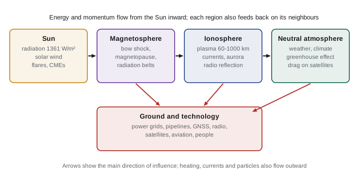
Look up on a clear winter night in Churchill or Yellowknife and you may see curtains of green light rippling a hundred kilometres overhead. The same night, a pilot on a polar flight may be told to fly a lower route, a power utility may be watching currents creep through its transformers, and the satellite navigation in a farmer's tractor may wander by several metres. All of these follow from one chain of physics that starts at the Sun, crosses 150 million kilometres of nearly empty space, compresses the Earth's magnetic field, dumps energy into a thin layer of charged gas at the top of the atmosphere, and finally reaches the ground. Atmospheric and space physics is the study of that chain. It joins thermodynamics and fluid mechanics, which govern the weather and climate of the lower atmosphere, to electromagnetism and plasma physics, which govern the ionosphere, the magnetosphere and the solar wind. This course takes them in that order, from the ground up, and ends with space weather, where all of them meet.

The regions of the system

It helps to name the regions before studying them. The neutral atmosphere is the gas we breathe, a mixture of nitrogen, oxygen, argon, water vapor and traces of carbon dioxide and other gases. It is held to the planet by gravity, its pressure falls roughly exponentially with height, and its temperature rises and falls in a pattern that divides it into the troposphere, stratosphere, mesosphere and thermosphere. Lesson 2 explains that pattern. Within the lowest 10 to 15 km, the troposphere, almost all the weather happens, driven by sunlight absorbed at the ground and carried upward by rising air and by evaporated water. Lessons 3 and 4 treat the thermodynamics and the dynamics of that air.

The atmosphere also controls the planet's energy balance. Sunlight arrives mostly at visible wavelengths, while the Earth radiates in the infrared, and the gases that absorb infrared, chiefly water vapor and carbon dioxide, keep the surface far warmer than it would otherwise be. Lessons 5 and 6 develop the radiative physics behind this greenhouse effect and use it to understand climate sensitivity: how much the surface warms when the infrared opacity of the air increases.

Above about 60 km, ultraviolet and X-ray photons from the Sun strip electrons from atoms and molecules, and a fraction of the gas becomes a plasma. This partly ionized region, the ionosphere, extends to about 1000 km and is the subject of lessons 7 and 8. Even though the charged particles are a tiny minority, they reflect radio waves, carry electric currents of a million amperes and more, and delay satellite navigation signals. Beyond the ionosphere, the Earth's magnetic field dominates the motion of charged particles out to about ten Earth radii on the day side and to hundreds of Earth radii on the night side. This region, the magnetosphere, holds the Van Allen radiation belts and is the subject of lesson 10. It exists because of the solar wind, a supersonic stream of plasma blowing off the Sun, which lesson 9 derives from the physics of the solar corona. Lesson 11 shows how the solar wind's energy enters the magnetosphere and lights up the aurora, and lesson 12 follows it all the way to power grids and satellites.

Scales that span many orders of magnitude

The physics changes from region to region because the numbers change enormously. At sea level the air presses with about \(10^5\) Pa and holds about \(2.5\times10^{25}\) molecules in every cubic metre. The solar wind at the Earth's orbit has about five protons per cubic centimetre and pushes on the magnetosphere with roughly one nanopascal. Between those extremes lies a factor of about \(10^{14}\) in pressure. In dense air, molecules collide billions of times a second and the gas behaves as a continuous fluid with a single temperature. In the solar wind a proton may travel an astronomical unit between collisions, and the gas behaves instead as a collection of charged particles tied to magnetic field lines. The ionosphere is in between: collisions with neutral atoms matter in its lower part and become negligible in its upper part.

The program below puts numbers on some of these scales. It weighs the whole atmosphere from the sea-level pressure, computes the temperature at which the Earth must radiate to balance the sunlight it absorbs, compares the pressure of the air with the ram pressure of the solar wind, gives the plasma frequency of the ionosphere at two typical densities, and lists some characteristic travel times.

import math
g = 9.81; RE = 6.371e6; p0 = 101325.0
area = 4 * math.pi * RE**2
mass_air = p0 * area / g
print(f"mass of the atmosphere = p0 * 4 pi RE^2 / g = {mass_air:.3e} kg")
print(f"air above each m^2 of ground = {p0 / g:,.0f} kg")

S0 = 1361.0; albedo = 0.30; sigma = 5.670374419e-8
Te = ((1 - albedo) * S0 / (4 * sigma)) ** 0.25
print(f"mean absorbed sunlight = {(1 - albedo) * S0 / 4:.1f} W/m^2, emission temperature = {Te:.1f} K")
print(f"observed mean surface temperature about 288 K, so the atmosphere adds about {288 - Te:.0f} K")

# Pressures from the ground to the solar wind
k = 1.380649e-23; mp = 1.67262192e-27
n_sw = 5e6; v_sw = 4.0e5
p_dyn = n_sw * mp * v_sw**2
print(f"solar wind ram pressure (5 per cm^3, 400 km/s) = {p_dyn * 1e9:.2f} nPa")
print(f"ratio of sea-level pressure to solar wind pressure = {p0 / p_dyn:.1e}")

# Plasma frequency of the daytime F2 peak
e = 1.602176634e-19; me = 9.1093837e-31; eps0 = 8.8541878188e-12
for ne in (1e11, 1e12):
    fp = math.sqrt(ne * e**2 / (eps0 * me)) / (2 * math.pi)
    print(f"electron density {ne:.0e} per m^3 -> plasma frequency {fp / 1e6:.2f} MHz")

# Time scales in the coupled system
for label, t in [("sound crosses the troposphere (12 km at 330 m/s)", 12e3 / 330),
                 ("air parcel circles the globe at 20 m/s", 2 * math.pi * RE / 20),
                 ("solar wind travels 1 AU at 400 km/s", 1.496e11 / 4e5),
                 ("light travels 1 AU", 1.496e11 / 2.998e8)]:
    print(f"{label}: {t:.3g} s = {t / 86400:.3g} days")

mass of the atmosphere = p0 * 4 pi RE^2 / g = 5.268e+18 kg
air above each m^2 of ground = 10,329 kg
mean absorbed sunlight = 238.2 W/m^2, emission temperature = 254.6 K
observed mean surface temperature about 288 K, so the atmosphere adds about 33 K
solar wind ram pressure (5 per cm^3, 400 km/s) = 1.34 nPa
ratio of sea-level pressure to solar wind pressure = 7.6e+13
electron density 1e+11 per m^3 -> plasma frequency 2.84 MHz
electron density 1e+12 per m^3 -> plasma frequency 8.98 MHz
sound crosses the troposphere (12 km at 330 m/s): 36.4 s = 0.000421 days
air parcel circles the globe at 20 m/s: 2e+06 s = 23.2 days
solar wind travels 1 AU at 400 km/s: 3.74e+05 s = 4.33 days
light travels 1 AU: 499 s = 0.00578 days

Several results reappear throughout the course. The sea-level pressure of 101 325 Pa is simply the weight of the air above each square metre, about 10 tonnes, so the whole atmosphere has a mass of about \(5.3\times10^{18}\) kg. That is less than a millionth of the Earth's mass, a thin skin over the planet. The emission temperature of about 255 K is what a body absorbing 238 W/m\(^2\) of sunlight must have to radiate the same power away as a blackbody. The measured mean surface temperature is about 288 K, so something keeps the surface about 33 K warmer than the planet's radiating temperature. That something is the infrared opacity of the atmosphere, and lessons 5 and 6 work out how it operates.

The solar wind ram pressure of 1.34 nPa is about \(10^{14}\) times smaller than sea-level pressure, yet it is enough to confine the Earth's magnetic field to a cavity about ten Earth radii across on the day side, as lesson 10 shows. The plasma frequencies of 3 to 9 MHz explain why shortwave radio signals in that range are reflected by the ionosphere while FM and satellite signals at 100 MHz and above pass through it. And the travel times set the pace of space weather: light from a solar flare reaches us in about eight minutes, while the plasma that carries a storm takes from about a day to four days.

Coupling between the regions

The word coupled matters. The regions do not simply sit one above the other; they exchange energy, momentum and particles in both directions. Ultraviolet sunlight absorbed in the thermosphere heats it to between 700 and 1500 K depending on solar activity, and that heating makes the thermosphere expand, increasing the drag on satellites in low orbit. During a geomagnetic storm, electric currents flowing along magnetic field lines from the magnetosphere close through the ionosphere, where they dissipate tens to hundreds of gigawatts as heat, again inflating the thermosphere. Gravity waves generated by thunderstorms and by wind blowing over mountains propagate upward, grow in amplitude as the air thins, and break in the mesosphere, depositing momentum that drives a circulation from one pole to the other. Ions from the ionosphere flow up magnetic field lines into the magnetosphere, where they can become the dominant population of the ring current during a storm. Climate change is coupled in the same way: increasing carbon dioxide warms the lower atmosphere but cools the stratosphere and thermosphere, because above the level where it traps heat, carbon dioxide mostly radiates energy away to space.

A short history

Measurements of the atmosphere began with Evangelista Torricelli's mercury barometer in 1643. In 1648, at Blaise Pascal's request, his brother-in-law carried a barometer up the Puy de Dôme in central France and found the mercury column shorter at the summit, showing that air pressure is the weight of the air above. In 1735 George Hadley explained the trade winds by the rising of warm air near the equator and the effect of the Earth's rotation, and in 1856 William Ferrel added the mid-latitude circulation. In 1902 Léon Teisserenc de Bort, using unmanned balloons, found that the temperature stops falling at about 11 km, discovering the stratosphere.

Space physics grew from the study of the aurora and of the Earth's magnetism. On 1 September 1859 Richard Carrington saw a brilliant white-light flare on the Sun, and about 17.6 hours later the largest magnetic storm in the historical record began, with aurora seen in the tropics and telegraph systems sparking and failing. Kristian Birkeland, after expeditions to northern Norway around 1900, proposed in 1908 that the aurora is driven by electric currents flowing along magnetic field lines. Guglielmo Marconi's transatlantic radio signal of December 1901 led Arthur Kennelly and Oliver Heaviside to propose in 1902 a conducting layer in the upper atmosphere, and Edward Appleton confirmed it by experiment in 1924. Eugene Parker predicted the supersonic solar wind in 1958, and in the same year James Van Allen's Geiger counter on Explorer 1, the first American satellite, found the radiation belts. Canada's first satellite, Alouette 1, launched in 1962, was built to sound the ionosphere from above, and it made Canada the third nation with a satellite in orbit.

Climate physics has a parallel history. Svante Arrhenius estimated in 1896 how much the Earth would warm if the carbon dioxide in the air doubled. Guy Callendar showed in 1938 that carbon dioxide was rising and that the Earth had warmed. Charles David Keeling began precise measurements at Mauna Loa in 1958, and the record of rising carbon dioxide he started is still running. Syukuro Manabe and Richard Wetherald built the first radiative-convective model with realistic absorption in 1967, finding a warming of about 2 K for doubled carbon dioxide, and Manabe shared the 2021 Nobel Prize in Physics for this work.

Canada and the high latitudes

The high latitudes are where much of this physics is most visible. The auroral zone, where aurora is seen most often, is a ring of magnetic latitude near 65 to 70 degrees, which passes over northern Canada: over Yellowknife, Churchill and the Hudson Bay region. Because the north magnetic pole lies in the Canadian Arctic, Canada sits under the auroral zone at lower geographic latitudes than Europe or Asia do. The country has a long tradition of upper-atmosphere research, from the Alouette and ISIS satellites to ground radars and optical networks, and the Canadian Space Weather Forecast Centre of Natural Resources Canada issues forecasts for the power, pipeline and satellite industries. In the United States the Space Weather Prediction Center of the National Oceanic and Atmospheric Administration, in Boulder, Colorado, plays the same role and issues the storm scales used in lesson 12.

Ground-based research sites illustrate the range of the subject. The PEARL laboratory near Eureka on Ellesmere Island, run by the CANDAC network, measures the Arctic atmosphere from the ground to the mesosphere. The SuperDARN radars, with Canadian stations operated from the University of Saskatchewan, map the flow of ionospheric plasma across the polar cap. The CASSIOPE satellite's ePOP instruments and the European Swarm satellites measure currents and fields above the ionosphere. In Alaska, the Poker Flat Research Range launches sounding rockets directly into auroral arcs.

How this course is organized

Lessons 2 to 4 treat the neutral atmosphere: its structure and hydrostatic balance, the thermodynamics of rising air, clouds and stability, and the dynamics of large-scale winds under the Earth's rotation. Lessons 5 and 6 treat radiation and climate: the transfer of radiation through an absorbing atmosphere, the greenhouse effect, radiative forcing, feedbacks and climate sensitivity. Lessons 7 and 8 treat the ionosphere: how photoionization builds its layers, and how it affects radio propagation and satellite navigation. Lessons 9 to 11 move outward to the Sun and the solar wind, the magnetosphere and its trapped particles, and the aurora and geomagnetic storms. The capstone, lesson 12, follows the effects of space weather into power grids, satellites, aviation and forecasting.

The course assumes the electromagnetism of PHYS-381 and PHYS-382, including the plasma frequency and ionospheric reflection met in PHYS-382, and the thermal physics of PHYS-261, whose capstone built a one-layer model of the Earth's energy balance. The Coriolis force from PHYS-244 returns in lesson 4. Every lesson includes runnable Python using only the standard library.