Cosmology I: the FLRW metric, Hubble's law and the Friedmann equations

General relativity is the first theory of gravity that can be applied to the universe as a whole. Newton's theory has no consistent answer to the question of what an infinite, uniform distribution of matter does; Einstein's equations give a precise one. In 1917 Einstein himself applied them to the cosmos and, believing the universe static, added the cosmological constant to hold it still. In 1922 Alexander Friedmann, a Russian mathematician and meteorologist, found that the equations naturally describe universes that expand or contract, and in 1927 Georges Lemaître, a Belgian priest and physicist, derived the same solutions independently and connected them to the redshifts of galaxies, deriving the linear relation between velocity and distance two years before Edwin Hubble's data made it famous. This lesson builds the standard cosmological model from two assumptions and the field equations. PHYS-430 introduced the expanding universe observationally; here we derive it.

The cosmological principle and the FLRW metric

On large enough scales, a few hundred million light-years and more, the universe looks the same everywhere and in every direction. Galaxy surveys show the distribution of matter becoming smooth on these scales, and the cosmic microwave background is the same temperature in every direction to one part in 100,000. The cosmological principle elevates this to an assumption: the universe is homogeneous and isotropic. With it, the most general metric is the Friedmann–Lemaître–Robertson–Walker metric,

Here \(t\) is cosmic time, measured by clocks moving with the average matter, and \((r, \theta, \phi)\) are comoving coordinates that label galaxies, fixed as the universe expands. All the dynamics is in the scale factor \(a(t)\), conventionally normalized to \(a = 1\) today, which multiplies every distance between comoving galaxies. The constant \(k\) describes the curvature of space at a fixed time: \(k = 0\) is flat Euclidean space, \(k > 0\) the three-dimensional surface of a hypersphere, finite but unbounded, and \(k < 0\) a hyperbolic space. The geometry of space and the expansion are logically separate; observations, as lesson 11 shows, find space flat to within half a part in a hundred.

Hubble's law and redshift

The proper distance to a comoving galaxy at coordinate \(r\) is \(d = a(t)\chi\), where \(\chi\) is the comoving distance. It changes at the rate \(\dot{d} = \dot{a}\chi = (\dot{a}/a)d\). This is Hubble's law, \(v = H d\), with the Hubble parameter

The law is exact in the FLRW metric for proper distances and their rates of change, and it holds for every observer: everyone sees the others receding, with no centre. Velocities can exceed \(c\) for distant enough galaxies, which does not violate relativity because no signal overtakes light locally; the distance is growing because space is expanding. A photon travelling between galaxies has its wavelength stretched with the expansion. Integrating the null geodesic in the FLRW metric shows that a wavelength emitted when the scale factor was \(a_e\) is received today stretched by

Redshift is a direct measure of how much the universe has expanded since the light left. A galaxy at redshift 1 emitted its light when the universe was half its present size; the microwave background at redshift 1,100 was emitted when it was a thousandth. The interpretation of cosmological redshift as a Doppler shift works only for small \(z\), where \(cz \approx H_0 d\).

The Friedmann equations

Inserting the FLRW metric into the Einstein equation, with matter described as a perfect fluid of density \(\rho\) and pressure \(p\), gives two equations. The first, from the 00 component, is the Friedmann equation:

The second, from the spatial components, is the acceleration equation:

The first can be understood with Newtonian physics. Consider a sphere of radius \(R = a\chi\) cut out of a uniform universe. By Newton's shell theorem, which Birkhoff's theorem in lesson 6 extends to general relativity, a test galaxy on its surface feels only the mass inside, \(M = \frac{4}{3}\pi R^3\rho\). Its energy per unit mass, \(\frac{1}{2}\dot{R}^2 - GM/R\), is constant; dividing by \(\frac{1}{2}R^2\) gives \(H^2 = \frac{8\pi G}{3}\rho + 2E/R^2\). The Newtonian energy constant becomes, in general relativity, the spatial curvature: a universe with negative energy, bound, has positive curvature. What Newton cannot supply is the pressure term in the acceleration equation: pressure gravitates, as lesson 5 showed, so a fluid with positive pressure decelerates the expansion more strongly than dust of the same density, and a fluid with \(p < -\rho c^2/3\) accelerates it.

Energy conservation, \(\nabla_\mu T^{\mu\nu} = 0\), gives the fluid equation \(\dot{\rho} + 3H(\rho + p/c^2) = 0\). For each component with equation of state \(p = w\rho c^2\), it implies \(\rho \propto a^{-3(1+w)}\). Three cases matter:

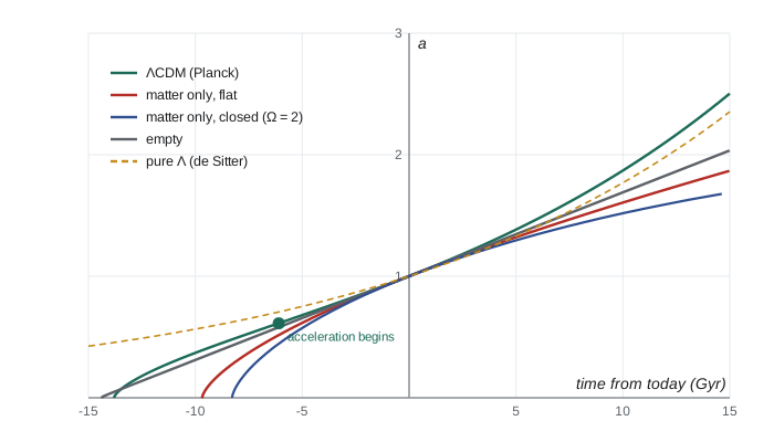
Because the three components dilute at different rates, each dominated in turn. In the early universe radiation dominated; around redshift 3,400, about 50,000 years after the Big Bang, matter took over; and about 3.5 billion years ago, at redshift 0.3, the cosmological constant came to dominate. The expansion had already begun to accelerate somewhat earlier, at redshift 0.63, about 6 billion years ago, when the vacuum energy's repulsion first outweighed the attraction of matter in the acceleration equation.

Density parameters

Dividing the Friedmann equation by \(H^2\) suggests measuring each component against the critical density, the density that would make space flat:

where \(\Omega_k = -kc^2/(a^2H^2)\) is the curvature contribution and \(\Omega_\Lambda = \Lambda c^2/(3H^2)\). For \(H_0 = 67.4\) km/s/Mpc the critical density is \(8.5 \times 10^{-27}\) kg/m³, about five hydrogen atoms per cubic metre. In terms of today's density parameters, the Friedmann equation becomes

The Planck satellite's 2018 results, combined with other data, give \(\Omega_m = 0.315\), \(\Omega_\Lambda = 0.685\), \(\Omega_k\) consistent with zero within about 0.002, and \(\Omega_r \approx 9 \times 10^{-5}\) from photons and neutrinos. The matter is mostly dark: ordinary atoms, baryons, contribute only \(\Omega_b = 0.049\). Lesson 12 discusses what the dark components might be.

Exact solutions

For a flat universe with a single component, the Friedmann equation can be solved directly. With matter only, the Einstein–de Sitter model, \(a \propto t^{2/3}\) and the age is \(t_0 = \frac{2}{3}H_0^{-1}\). With radiation only, \(a \propto t^{1/2}\) and \(t_0 = \frac{1}{2}H_0^{-1}\). With a cosmological constant only, the de Sitter model, \(a \propto e^{Ht}\) with constant \(H\): exponential expansion with no beginning. For the real mixture the age is an integral,

which must be evaluated numerically. The Hubble time \(1/H_0\) is 14.5 billion years for \(H_0 = 67.4\); the deceleration during the matter era and the acceleration since nearly cancel, giving an age close to \(1/H_0\).

import math
Mpc_km, Gyr_s = 3.0857e19, 3.156e16
G = 6.674e-11
def E(a, Om, Ol, Or):
    Ok = 1 - Om - Ol - Or
    return math.sqrt(Or / a**4 + Om / a**3 + Ok / a**2 + Ol)
def age(H0, Om, Ol, Or=9.1e-5, a_end=1.0, n=40000):
    # integrate dt = da / (a H); substitute a = x^2 to tame the small-a end
    H0s = H0 / Mpc_km
    total = 0.0
    xs = math.sqrt(a_end)
    for i in range(n):
        x = (i + 0.5) * xs / n
        a = x * x
        total += 2 * x / (a * H0s * E(a, Om, Ol, Or)) * xs / n
    return total / Gyr_s
H0 = 67.4
print(f"Hubble time 1/H0 = {Mpc_km/H0/Gyr_s:.2f} Gyr")
print(f"critical density = {3*(H0/Mpc_km)**2/(8*math.pi*G):.3e} kg/m^3")
for name, Om, Ol in (("Planck LCDM", 0.315, 0.685), ("matter only (EdS)", 1.0, 0.0),
                     ("open, matter 0.3", 0.3, 0.0), ("closed, matter 2", 2.0, 0.0)):
    print(f"{name:18s}: age {age(H0, Om, Ol):6.2f} Gyr")
# lookback time and the age of the universe at various redshifts in LCDM
t0 = age(H0, 0.315, 0.685)
for z in (0.3, 1, 3, 10, 1100):
    a = 1 / (1 + z)
    ta = age(H0, 0.315, 0.685, a_end=a)
    print(f"z = {z:5}: universe then {ta*1e3 if ta < 1 else ta:8.3f} {'Myr' if ta < 1 else 'Gyr'}, lookback {t0-ta:6.2f} Gyr")
# when did acceleration begin? q = 0 where Om a^-3 = 2 Ol
a_acc = (0.315 / (2 * 0.685)) ** (1/3)
print(f"acceleration began at z = {1/a_acc - 1:.2f}, {t0 - age(H0, 0.315, 0.685, a_end=a_acc):.2f} Gyr ago")

Hubble time 1/H0 = 14.51 Gyr
critical density = 8.533e-27 kg/m^3
Planck LCDM       : age  13.79 Gyr
matter only (EdS) : age   9.67 Gyr
open, matter 0.3  : age  11.73 Gyr
closed, matter 2  : age   8.28 Gyr
z =   0.3: universe then   10.251 Gyr, lookback   3.54 Gyr
z =     1: universe then    5.841 Gyr, lookback   7.95 Gyr
z =     3: universe then    2.138 Gyr, lookback  11.65 Gyr
z =    10: universe then  470.092 Myr, lookback  13.32 Gyr
z =  1100: universe then    0.366 Myr, lookback  13.79 Gyr
acceleration began at z = 0.63, 6.10 Gyr ago

The \(\Lambda\)CDM model gives an age of 13.8 billion years, consistent with the oldest stars, whose ages from stellar evolution are around 12 to 13 billion years. The matter-only model, which was the standard expectation before 1998, gives only 9.7 billion years for the same Hubble constant, younger than the oldest stars, a tension that was one of the clues to dark energy. The universe was about 370,000 years old when the microwave background was released at redshift 1,100, and only about half a billion years old at redshift 10, where JWST has found galaxies in surprising numbers.

Distances in an expanding universe

In an expanding universe there are several useful distances, all equal for nearby objects but different far away. The comoving distance \(\chi = c\int_0^z dz'/H(z')\) is today's proper distance to a galaxy at redshift \(z\). The luminosity distance \(d_L\), defined so that flux \(F = L/(4\pi d_L^2)\), is \(d_L = (1 + z)\chi\) in a flat universe: one factor of \(1 + z\) because each photon is redshifted, another because photons arrive spread out in time. The angular diameter distance \(d_A = \chi/(1 + z)\), defined so that an object of size \(D\) subtends \(D/d_A\), has the curious property of reaching a maximum near redshift 1.6 and then decreasing: very distant objects look larger in angle because we see them as they were when the universe was small.

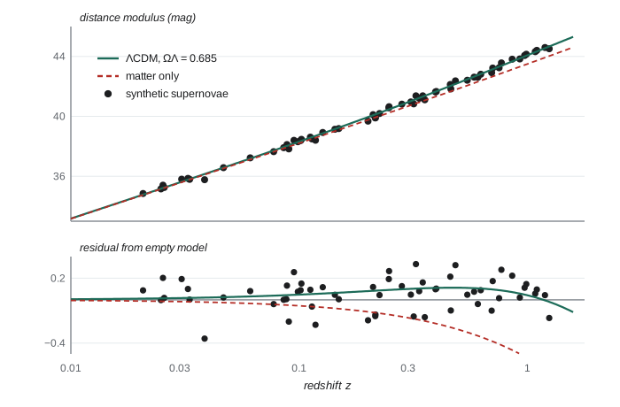
Type Ia supernovae, thermonuclear explosions of white dwarfs whose peak luminosity can be calibrated from their light-curve shapes, are standard candles bright enough to be seen across billions of light-years. In 1998 two teams, the Supernova Cosmology Project led by Saul Perlmutter and the High-z Supernova Search Team led by Brian Schmidt and Adam Riess, found that distant supernovae are about 25 parts in a hundred fainter than expected in a decelerating universe: they are farther away, because the expansion has been accelerating. The three shared the 2011 Nobel Prize in Physics. The code below fits synthetic supernova data, generated from the Planck model with realistic scatter, to determine \(\Omega_\Lambda\) in a flat universe.

import math, random
random.seed(1998)
c = 299792.458
def dL(z, Om, H0=70.0, n=400):          # flat universe, Mpc
    Ol = 1 - Om
    s = 0.0
    for i in range(n):
        zz = (i + 0.5) * z / n
        s += 1 / math.sqrt(Om * (1 + zz)**3 + Ol) * z / n
    return (1 + z) * c / H0 * s
def mu(z, Om): return 5 * math.log10(dL(z, Om)) + 25
data = []
for i in range(60):
    z = 10 ** random.uniform(-1.7, 0.15)
    data.append((z, mu(z, 0.315) + random.gauss(0, 0.15)))
def chi2(Om):
    # marginalize the unknown absolute calibration analytically: best offset is the mean residual
    r = [m - mu(z, Om) for z, m in data]
    off = sum(r) / len(r)
    return sum((x - off) ** 2 for x in r) / 0.15**2
grid = [i / 100 for i in range(5, 101)]
best = min(grid, key=chi2)
c_best = chi2(best)
inside = [Om for Om in grid if chi2(Om) < c_best + 1]
print(f"best fit Omega_m = {best:.2f}, Omega_Lambda = {1-best:.2f}")
print(f"1-sigma range of Omega_m: {min(inside):.2f} to {max(inside):.2f}")
print(f"chi^2 at best fit {c_best:.1f} for {len(data)-2} degrees of freedom; matter-only chi^2 {chi2(1.0):.1f}")
print(f"at z = 0.5 an LCDM supernova is {mu(0.5,0.315)-mu(0.5,1.0):.2f} mag fainter than in a matter-only universe")

best fit Omega_m = 0.29, Omega_Lambda = 0.71
1-sigma range of Omega_m: 0.25 to 0.33
chi^2 at best fit 50.9 for 58 degrees of freedom; matter-only chi^2 152.9
at z = 0.5 an LCDM supernova is 0.39 mag fainter than in a matter-only universe