The hydrogen atom revisited: fine structure, the Zeeman effect and hyperfine splitting

The exact solution of hydrogen in PHYS-372 used the Hamiltonian \(H^0 = p^2/2m - e^2/4\pi\varepsilon_0 r\). It predicted energies that depend only on \(n\), with \(2n^2\) states in each level once spin is counted. This lesson adds, one at a time, the corrections that real hydrogen requires and shows how perturbation theory, ordinary and degenerate, turns each into a measurable splitting. The tools are those of lessons 2, 3 and 6: spin, coupled angular momentum states and the first-order formula \(E^1 = \langle H'\rangle\), applied in a basis of good quantum numbers.

The relativistic kinetic energy

The kinetic energy of a relativistic particle is \(T = \sqrt{p^2c^2 + m^2c^4} - mc^2\). Expanding in powers of \(p/mc\),

The \(n\)th level is \(2n^2\)-fold degenerate, so in principle degenerate perturbation theory is needed. But \(H'_{\text{r}}\) is spherically symmetric and does not involve spin, so it commutes with \(L^2\), \(L_z\) and \(S_z\); the standard states \(|n\ell m_\ell m_s\rangle\) are already good states and the non-degenerate formula applies. The calculation is neat. Write \(p^4/8m^3c^2 = (1/2mc^2)(p^2/2m)^2\) and use \(p^2/2m = E_n + e^2/4\pi\varepsilon_0 r\) from the unperturbed Schrödinger equation. Then

using the hydrogen expectation values \(\langle 1/r\rangle = 1/n^2a\) and \(\langle 1/r^2\rangle = 1/[(\ell + \tfrac12)n^3a^2]\), which follow from the radial functions of PHYS-372. The correction lowers every level by a few parts in \(10^5\) of its energy, more for small \(\ell\) because those orbits come closer to the nucleus where the electron moves fastest.

Spin–orbit coupling

In the rest frame of the electron, the proton circles it and produces a magnetic field \(\mathbf B\) proportional to the orbital angular momentum. The electron's magnetic moment \(\boldsymbol\mu = -(e/m)\mathbf S\) has energy \(-\boldsymbol\mu\cdot\mathbf B\) in this field. A careful treatment includes Thomas precession, a kinematic effect of the electron's accelerated frame found by Llewellyn Thomas in 1926, which halves the naive result:

Now \(\mathbf S\cdot\mathbf L\) does not commute with \(L_z\) or \(S_z\), so the product states are not good states. It does commute with \(L^2\), \(S^2\), \(J^2\) and \(J_z\), so the coupled states \(|n\ell j m_j\rangle\) of lesson 3 are. In them \(\mathbf S\cdot\mathbf L = \tfrac12\hbar^2[j(j+1) - \ell(\ell+1) - \tfrac34]\), and with \(\langle 1/r^3\rangle = 1/[\ell(\ell + \tfrac12)(\ell + 1)n^3a^3]\),

The fine-structure formula

Adding the two corrections, for \(j = \ell \pm \tfrac12\), the \(\ell\) dependence cancels in a remarkable way, leaving a result that depends only on \(n\) and \(j\):

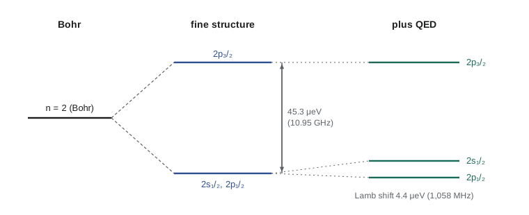
For \(\ell = 0\), where the spin–orbit term vanishes, a third correction, the Darwin term, arising from the electron's relativistic jitter, contributes exactly what the formula needs, so the result holds for all \(\ell\). It is also exactly what the Dirac equation gives when expanded to order \(\alpha^4\), a fine confirmation of the whole approach. The fine structure lifts the degeneracy in \(\ell\) only partly: states with the same \(n\) and \(j\) but different \(\ell\), such as \(2s_{1/2}\) and \(2p_{1/2}\), remain degenerate. Every level is lowered, and the \(n = 2\) level splits into two, \(2p_{3/2}\) above the degenerate pair \(2s_{1/2}\), \(2p_{1/2}\), separated by \(45.3\) micro-electronvolts, a frequency of 10.95 GHz.

The Lamb shift

In 1947 Willis Lamb and Robert Retherford at Columbia University used microwaves to drive transitions between the \(n = 2\) levels of a beam of hydrogen atoms and found that \(2s_{1/2}\) lies above \(2p_{1/2}\) by about 1,058 MHz, or \(4.4 \times 10^{-6}\) eV, in conflict with the Dirac equation. Hans Bethe's estimate the same year, treating the electron's interaction with the zero-point fluctuations of the electromagnetic field, explained most of it and launched modern quantum electrodynamics. The Lamb shift is of order \(\alpha^5 mc^2\) and is a pure field-theory effect, beyond the quantum mechanics of this course; Lamb received the Nobel Prize in 1955.

The Zeeman effect

An external magnetic field \(\mathbf B_{\text{ext}} = B\hat{\mathbf z}\) couples to both the orbital and spin magnetic moments:

with the electron's \(g \approx 2\) doubling the spin term. How to treat it depends on its size compared with the fine structure.

In a weak field, \(\mu_B B \ll E_{\text{fs}}\), the fine structure dominates and the good states are \(|n\ell j m_j\rangle\). The Zeeman term is the perturbation, and its first-order shift requires \(\langle L_z + 2S_z\rangle = \langle J_z + S_z\rangle\) in a coupled state. The vector model of lesson 3 gives the answer: \(\mathbf S\) precesses rapidly about \(\mathbf J\), so only its projection on \(\mathbf J\) survives, \(\langle\mathbf S\rangle = (\langle\mathbf S\cdot\mathbf J\rangle/J^2)\,\mathbf J\). This leads to

where \(g_J\) is the Landé \(g\)-factor, introduced by Alfred Landé in 1921 from spectra. Each level splits into \(2j + 1\) equally spaced components whose spacing depends on \(\ell\) and \(j\), not just on \(B\). For \(2s_{1/2}\), \(g_J = 2\); for \(2p_{1/2}\), \(2/3\); for \(2p_{3/2}\), \(4/3\). Spectral lines therefore split into patterns of more than the three components that orbital motion alone would give, the anomalous Zeeman effect that puzzled physicists until spin was understood.

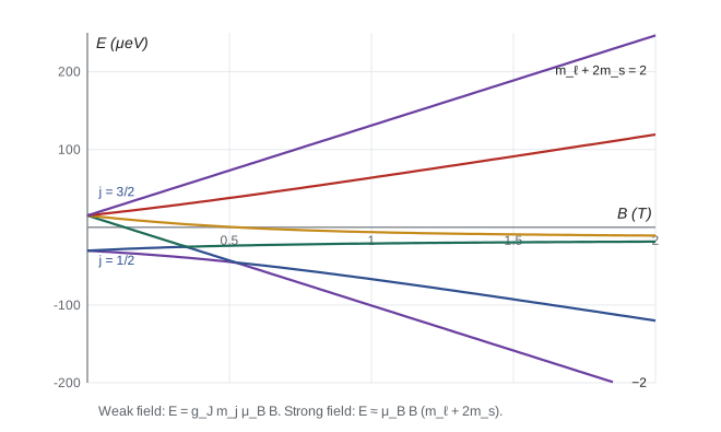
In a strong field, \(\mu_B B \gg E_{\text{fs}}\), the Zeeman term dominates. The good states are the product states \(|n\ell m_\ell m_s\rangle\), the energies are \(\mu_B B(m_\ell + 2m_s)\), and the fine structure becomes a small correction. This is the Paschen–Back effect, observed by Friedrich Paschen and Ernst Back in 1912. Between the two limits, neither basis diagonalizes the Hamiltonian, and one must diagonalize the full matrix of \(H'_{\text{so}} + H'_Z\) within the level. The program does this for the six states of hydrogen \(2p\).

import math
alpha = 1 / 137.035999
mc2 = 510998.95          # electron rest energy, eV
Ry = 13.605693           # eV
muB = 5.7883818e-5       # Bohr magneton, eV per tesla

def E_fine(n, j):
    """Bohr energy plus the fine-structure correction (relativistic + spin-orbit + Darwin)."""
    En = -Ry / n ** 2
    return En + (-En * alpha ** 2 / n ** 2) * (3 / 4 - n / (j + 0.5))

print("Fine structure of hydrogen (shift from the Bohr energy, micro-eV)")
for n in (1, 2, 3):
    for j in [k + 0.5 for k in range(n)]:
        print(f"  n = {n}, j = {j:3.1f}: {1e6 * (E_fine(n, j) + Ry / n ** 2):+9.2f}")
split2 = E_fine(2, 1.5) - E_fine(2, 0.5)
print(f"  2p3/2 - 2p1/2 splitting: {split2 * 1e6:.2f} micro-eV = {split2 / 4.135667696e-15 / 1e9:.3f} GHz")
print()

def lande(l, s, j): return 1 + (j * (j + 1) - l * (l + 1) + s * (s + 1)) / (2 * j * (j + 1))
for name, l, j in (("2s1/2", 0, 0.5), ("2p1/2", 1, 0.5), ("2p3/2", 1, 1.5)):
    print(f"  Lande g for {name}: {lande(l, 0.5, j):.4f}")
print()

def jacobi(A, sweeps=50):
    n = len(A); A = [r[:] for r in A]
    for _ in range(sweeps):
        for p in range(n - 1):
            for q in range(p + 1, n):
                if abs(A[p][q]) < 1e-18: continue
                th = 0.5 * math.atan2(2 * A[p][q], A[q][q] - A[p][p]); c, s = math.cos(th), math.sin(th)
                for k in range(n):
                    A[k][p], A[k][q] = c * A[k][p] - s * A[k][q], s * A[k][p] + c * A[k][q]
                for k in range(n):
                    A[p][k], A[q][k] = c * A[p][k] - s * A[q][k], s * A[p][k] + c * A[q][k]
    return sorted(A[i][i] for i in range(n))

# 2p manifold in the product basis |ml, ms>: H = A L.S/hbar^2 + muB B (Lz + 2 Sz)/hbar
Aso = split2 / 1.5
basis = [(ml, ms) for ml in (1, 0, -1) for ms in (0.5, -0.5)]
def H2p(B):
    H = [[0.0] * 6 for _ in range(6)]
    for i, (ml, ms) in enumerate(basis):
        H[i][i] = Aso * ml * ms + muB * B * (ml + 2 * ms)
        for k, (ml2, ms2) in enumerate(basis):     # (L+ S- + L- S+)/2 terms
            if ml2 == ml + 1 and ms2 == ms - 1:
                H[k][i] = H[i][k] = 0.5 * Aso * math.sqrt(2 - ml * (ml + 1)) * math.sqrt(0.75 - ms * (ms - 1))
    return H
print("Hydrogen 2p levels in a magnetic field (micro-eV, from the 2p centroid)")
for B in (0.0, 0.05, 0.5, 5.0):
    print(f"  B = {B:4.2f} T: " + "  ".join(f"{1e6 * e:+8.1f}" for e in jacobi(H2p(B))))
print(f"  weak field at 0.05 T, 2p3/2 slopes g mj muB B: " +
      "  ".join(f"{1e6 * (Aso / 2 + lande(1, .5, 1.5) * mj * muB * 0.05):+8.1f}" for mj in (-1.5, -0.5, 0.5, 1.5)))
print()
gp, me_mp = 5.5856947, 1 / 1836.15267
dE = (4 / 3) * gp * me_mp * alpha ** 4 * mc2      # ground-state hyperfine splitting, F = 1 minus F = 0
print(f"hyperfine splitting of 1s: {dE * 1e6:.3f} micro-eV, frequency {dE / 4.135667696e-15 / 1e6:.0f} MHz, wavelength {2.99792458e8 / (dE / 4.135667696e-15) * 100:.2f} cm")

Fine structure of hydrogen (shift from the Bohr energy, micro-eV)
  n = 1, j = 0.5:   -181.13
  n = 2, j = 0.5:    -56.60
  n = 2, j = 1.5:    -11.32
  n = 3, j = 0.5:    -20.13
  n = 3, j = 1.5:     -6.71
  n = 3, j = 2.5:     -2.24
  2p3/2 - 2p1/2 splitting: 45.28 micro-eV = 10.949 GHz

  Lande g for 2s1/2: 2.0000
  Lande g for 2p1/2: 0.6667
  Lande g for 2p3/2: 1.3333

Hydrogen 2p levels in a magnetic field (micro-eV, from the 2p centroid)
  B = 0.00 T:    -30.2     -30.2     +15.1     +15.1     +15.1     +15.1
  B = 0.05 T:    -31.2     -29.3      +9.3     +13.2     +17.1     +20.9
  B = 0.50 T:    -44.5     -42.8     -23.7      +0.4     +37.6     +73.0
  B = 5.00 T:   -563.7    -291.1     -16.6     -13.4    +290.9    +593.9
  weak field at 0.05 T, 2p3/2 slopes g mj muB B:     +9.3     +13.2     +17.0     +20.9

hyperfine splitting of 1s: 5.877 micro-eV, frequency 1421 MHz, wavelength 21.09 cm

At zero field the \(2p\) levels sit at \(-30.2\) and \(+15.1\) micro-eV about their centroid, the \(j = 1/2\) pair and the \(j = 3/2\) quartet. At 0.05 T the four upper levels are evenly spaced by \(g_J\mu_B B = 3.9\) micro-eV, matching the weak-field formula to the printed precision. By 5 T the levels have reorganized into the Paschen–Back pattern, close to \(\mu_B B(m_\ell + 2m_s)\) with values \(\pm 2\), \(\pm 1\) and \(0\) times 289 micro-eV. The crossover occurs near half a tesla, where the Zeeman energy equals the fine-structure splitting.

Hyperfine structure and the 21 cm line

The proton has spin one-half and a magnetic moment \(\boldsymbol\mu_p = (g_pe/2m_p)\mathbf S_p\), with \(g_p = 5.59\). Its field acts on the electron's magnetic moment. For the ground state, where the electron's wave function is spherically symmetric, only a contact term survives, and first-order perturbation theory gives an energy proportional to \(\mathbf S_p\cdot\mathbf S_e\). Lesson 3 showed that this splits the triplet from the singlet. The result is

with the triplet above the singlet. A photon emitted when the electron's spin flips relative to the proton's has a frequency of 1,420 MHz and a wavelength of 21 cm. The program's estimate, 1,421 MHz, differs from the measured 1,420.4058 MHz by small corrections, mainly the anomalous moment of the electron. The transition is extraordinarily slow, with a lifetime of about ten million years, but interstellar space contains so much atomic hydrogen that the line is bright. Harold Ewen and Edward Purcell first detected it from the Milky Way in 1951, and mapping it revealed the spiral arms of the galaxy. Canada's CHIME telescope at the Dominion Radio Astrophysical Observatory in British Columbia maps redshifted 21 cm emission from the distant universe to trace its expansion.