Time-independent perturbation theory: non-degenerate and degenerate

Very few Hamiltonians can be diagonalized exactly. But many real problems are close to one that can: hydrogen with a weak applied field, an oscillator with a slightly anharmonic potential, an atom with small relativistic corrections. Perturbation theory is the systematic way to exploit that closeness. It expresses the energies and states of the full problem as power series in the strength of the extra term, with coefficients built entirely from the solutions of the simple problem. Developed by Erwin Schrödinger in 1926, in the third of his papers on wave mechanics, it is probably the most used calculation method in quantum physics.

Setting up the expansion

Suppose the Hamiltonian is \(H = H^0 + \lambda H'\), where the eigenvalue problem for \(H^0\) is solved, \(H^0\psi_n^0 = E_n^0\psi_n^0\), with orthonormal eigenstates, and \(\lambda\) is a bookkeeping parameter that will be set to 1 at the end. We look for the eigenstates and eigenvalues of \(H\) as power series:

Substituting into \(H\psi_n = E_n\psi_n\) and collecting powers of \(\lambda\) gives a hierarchy of equations. At order \(\lambda^0\) we recover the unperturbed problem. At order \(\lambda^1\):

First-order energy

Take the inner product of this equation with \(\psi_n^0\). Because \(H^0\) is Hermitian, \(\langle\psi_n^0|H^0\psi_n^1\rangle = E_n^0\langle\psi_n^0|\psi_n^1\rangle\), which cancels the matching term on the right. What remains is the central result of first-order perturbation theory:

The first-order correction to an energy is the expectation value of the perturbation in the unperturbed state. It is often all that is needed, and it is easy to evaluate. For example, if a box of width \(a\) has its floor raised by \(V_0\) over its left half, every level is raised to first order by \(V_0/2\), because each infinite-well eigenstate spends exactly half its probability in each half. For helium's ground state in lesson 1, taking the electron repulsion as \(H'\) gave a first-order correction of \(\tfrac54 Z \times 13.6\) eV = 34.0 eV, which raised the energy from \(-108.8\) to \(-74.8\) eV.

First-order state

To find the correction to the state, expand \(\psi_n^1\) in the complete set of unperturbed states, \(\psi_n^1 = \sum_{m \ne n} c_m\psi_m^0\). (A component along \(\psi_n^0\) itself can be removed by a change of normalization and phase, so it is set to zero.) Taking the inner product of the first-order equation with \(\psi_m^0\), \(m \ne n\), gives \((E_m^0 - E_n^0)c_m + \langle\psi_m^0|H'|\psi_n^0\rangle = 0\), so

The perturbation mixes into \(\psi_n^0\) a little of each other state, with an amplitude equal to the matrix element divided by the energy difference. Nearby states mix most. The formula fails when some \(E_m^0 = E_n^0\) with a nonzero matrix element: this is the degenerate case, treated below.

Second-order energy

Collecting terms of order \(\lambda^2\) and again projecting onto \(\psi_n^0\) gives \(E_n^2 = \langle\psi_n^0|H'|\psi_n^1\rangle\). Substituting the first-order state,

Two features of this formula are worth remembering. For the ground state, every denominator \(E_0^0 - E_m^0\) is negative, so the second-order correction to the ground-state energy is always negative or zero. And each pair of levels pushes the other away: if \(m\) lies above \(n\), its contribution lowers \(E_n\), and the matching term in \(E_m^2\) raises \(E_m\). This level repulsion is a general feature of quantum spectra. The second-order correction matters whenever the first order vanishes by symmetry, as for an atom in an electric field when the state has definite parity: the first-order shift \(\langle\psi|ez|\psi\rangle\) is zero, and the leading effect is the quadratic Stark shift, \(E^2 = -\tfrac12\alpha_{\text{pol}}\mathcal E^2\), which defines the atomic polarizability \(\alpha_{\text{pol}}\).

How good is it? The anharmonic oscillator

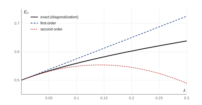
Consider the oscillator with a quartic correction, \(H = p^2/2m + \tfrac12 m\omega^2x^2 + \lambda x^4\), in units where \(\hbar = m = \omega = 1\). The ladder operators of PHYS-372 make the matrix elements easy: \(x = (a_+ + a_-)/\sqrt2\), so \(x^4\) connects \(|n\rangle\) to \(|n\rangle\), \(|n \pm 2\rangle\) and \(|n \pm 4\rangle\). For the ground state, \(\langle 0|x^4|0\rangle = 3/4\), so \(E_0^1 = 3\lambda/4\). The second-order sum has two terms, from \(|2\rangle\) with \(\langle 2|x^4|0\rangle = 3/\sqrt2\) and from \(|4\rangle\) with \(\langle 4|x^4|0\rangle = \sqrt6/2\):

So \(E_0 \approx \tfrac12 + \tfrac34\lambda - \tfrac{21}{8}\lambda^2\). The program compares this with the exact ground state, found by writing \(H\) as a matrix in the first 30 oscillator states and diagonalizing it with Jacobi rotations.

import math

def jacobi_eigenvalues(A, sweeps=60):
    """Eigenvalues of a real symmetric matrix by cyclic Jacobi rotations."""
    n = len(A); A = [row[:] for row in A]
    for _ in range(sweeps):
        off = sum(A[i][j] ** 2 for i in range(n) for j in range(n) if i != j)
        if off < 1e-22: break
        for p in range(n - 1):
            for q in range(p + 1, n):
                if abs(A[p][q]) < 1e-15: continue
                th = 0.5 * math.atan2(2 * A[p][q], A[q][q] - A[p][p])
                c, s = math.cos(th), math.sin(th)
                for k in range(n):
                    akp, akq = A[k][p], A[k][q]
                    A[k][p], A[k][q] = c * akp - s * akq, s * akp + c * akq
                for k in range(n):
                    apk, aqk = A[p][k], A[q][k]
                    A[p][k], A[q][k] = c * apk - s * aqk, s * apk + c * aqk
    return sorted(A[i][i] for i in range(n))

N = 36                                   # oscillator basis states kept (units hbar = m = omega = 1)
X = [[0.0] * N for _ in range(N)]
for n in range(N - 1):
    X[n][n + 1] = X[n + 1][n] = math.sqrt((n + 1) / 2)
mul = lambda A, B: [[sum(A[i][k] * B[k][j] for k in range(N)) for j in range(N)] for i in range(N)]
X2 = mul(X, X); X4 = mul(X2, X2)
print("Anharmonic oscillator H = p^2/2 + x^2/2 + lam x^4, ground-state energy")
print("   lam     exact     1st order  2nd order   error of 2nd order")
for lam in (0.01, 0.05, 0.1, 0.2):
    # keep the top of the truncated basis out of the x^4 matrix, where truncation corrupts it
    M = 30
    H = [[(i + 0.5 if i == j else 0.0) + lam * X4[i][j] for j in range(M)] for i in range(M)]
    E = jacobi_eigenvalues(H)[0]
    e1 = 0.5 + 0.75 * lam
    e2 = e1 - 21 / 8 * lam ** 2
    print(f"  {lam:5.2f}  {E:9.6f}  {e1:9.6f}  {e2:9.6f}   {e2 - E:+.2e}")
print()
# degenerate perturbation theory: linear Stark effect in hydrogen n = 2, basis (2s, 2p0)
a0, F = 5.29177e-11, 1.0e7           # Bohr radius in m, field in V/m
W = -3 * a0 * F                      # <2s| e F z |2p0> in eV, since e*F*z with z in m gives eV
print("Linear Stark effect, hydrogen n = 2, field 1.0e7 V/m (degenerate 2s, 2p0 pair)")
H = [[0.0, W], [W, 0.0]]
for e in jacobi_eigenvalues(H):
    print(f"  shift {e * 1e3:+.4f} meV")
print(f"  splitting 6 e a0 F = {6 * a0 * F * 1e3:.4f} meV; 2p(m = +1) and 2p(m = -1) unshifted")

Anharmonic oscillator H = p^2/2 + x^2/2 + lam x^4, ground-state energy
   lam     exact     1st order  2nd order   error of 2nd order
   0.01   0.507256   0.507500   0.507237   -1.87e-05
   0.05   0.532643   0.537500   0.530937   -1.71e-03
   0.10   0.559146   0.575000   0.548750   -1.04e-02
   0.20   0.602405   0.650000   0.545000   -5.74e-02

Linear Stark effect, hydrogen n = 2, field 1.0e7 V/m (degenerate 2s, 2p0 pair)
  shift -1.5875 meV
  shift +1.5875 meV
  splitting 6 e a0 F = 3.1751 meV; 2p(m = +1) and 2p(m = -1) unshifted

For \(\lambda = 0.01\), second order is within \(2 \times 10^{-5}\) of the exact energy. By \(\lambda = 0.1\) the error has grown to \(10^{-2}\), and at \(\lambda = 0.2\) the second-order result is worse than the first. The series for this problem is in fact divergent for every nonzero \(\lambda\), as Carl Bender and Tai Tsun Wu showed in 1969: the coefficients grow factorially, so adding more terms helps only up to a point. Perturbation series in physics are often asymptotic rather than convergent; used sensibly, keeping only the terms that are still getting smaller, they are nonetheless extremely accurate when the coupling is weak. Quantum electrodynamics, where the expansion parameter is \(\alpha/\pi \approx 0.002\), is the outstanding example.

Degenerate perturbation theory

When the unperturbed level is degenerate, say \(H^0\psi_a^0 = E^0\psi_a^0\) and \(H^0\psi_b^0 = E^0\psi_b^0\) with \(\langle\psi_a^0|\psi_b^0\rangle = 0\), the formula for \(\psi^1\) has a zero denominator. The way out is to recognize that any combination \(\alpha\psi_a^0 + \beta\psi_b^0\) is an equally good unperturbed state, and the perturbation selects particular combinations. Projecting the first-order equation onto \(\psi_a^0\) and \(\psi_b^0\) gives a 2 by 2 eigenvalue problem:

For an \(n\)-fold degenerate level the same recipe applies with an \(n\) by \(n\) matrix: the first-order energies are the eigenvalues of the perturbation restricted to the degenerate subspace, and its eigenvectors are the correct zeroth-order states, the good states. Often symmetry finds them without any calculation. If some Hermitian operator \(A\) commutes with both \(H^0\) and \(H'\), and the degenerate states have distinct eigenvalues of \(A\), then \(H'\) cannot connect them, the matrix \(W\) is already diagonal in the eigenbasis of \(A\), and ordinary non-degenerate formulas apply within each eigenvalue of \(A\). The labels of \(A\) are then called good quantum numbers. Lesson 7 uses exactly this argument for the fine structure: the spin–orbit term commutes with \(J^2\) and \(J_z\) but not with \(L_z\) and \(S_z\), so \(j\) and \(m_j\) are good quantum numbers and \(m_\ell\) and \(m_s\) are not.

The linear Stark effect

The classic example of degenerate perturbation theory is hydrogen's \(n = 2\) level in an electric field \(\mathcal E\) along \(z\), with \(H' = e\mathcal Ez\). The four spatial states \(2s, 2p_0, 2p_{+1}, 2p_{-1}\) are degenerate. Because \(H'\) commutes with \(L_z\), it connects only states with the same \(m\), and because \(z\) is odd under parity, its diagonal elements vanish. The only nonzero matrix element is \(\langle 2s|e\mathcal Ez|2p_0\rangle = -3e\mathcal Ea_0\), found from the hydrogen wave functions of PHYS-372. The 2 by 2 problem then gives first-order shifts \(\pm3e\mathcal Ea_0\) for the combinations \((2s \mp 2p_0)/\sqrt2\), while the \(m = \pm1\) states are unshifted. The good states are mixtures of different parity with a permanent electric dipole moment of \(3ea_0\). Unlike almost any other atom, hydrogen therefore shows a Stark shift linear in the field, a direct consequence of its accidental \(\ell\)-degeneracy. Johannes Stark discovered the splitting in 1913 and it was among the first successes of wave mechanics in 1926. For a field of \(10^7\) V/m the program gives a splitting of 3.2 meV.