Scattering theory: partial waves and the Born approximation

Much of what physicists know about the structure of matter came from scattering experiments. Ernest Rutherford found the atomic nucleus in 1911 by scattering alpha particles from gold foil. Electron scattering at Stanford in the 1950s measured the sizes of nuclei and protons, and deep inelastic scattering in 1968 revealed quarks inside the proton. Neutron scattering maps the arrangement and motion of atoms in materials, and X-ray scattering at synchrotrons such as the Canadian Light Source in Saskatoon and the Advanced Photon Source near Chicago determines the structures of proteins. This lesson sets up the quantum theory of scattering from a fixed potential and develops its two main tools: the partial-wave method, exact in principle and best at low energies, and the Born approximation, best at high energies and for weak potentials.

The scattering problem

A beam of particles of momentum \(\hbar k\) along \(z\) meets a potential \(V(r)\) localized near the origin. Far from the target, the stationary scattering state consists of the incident plane wave plus an outgoing spherical wave whose amplitude depends on direction:

The function \(f(\theta, \phi)\), the scattering amplitude, contains all the information an experiment can measure. The flux of the incident wave is \(|A|^2\hbar k/m\) per unit area; the flux through a distant detector subtending solid angle \(d\Omega\) is \(|A|^2|f|^2(\hbar k/m)\,d\Omega\). Their ratio is the differential cross-section, an effective target area for scattering into that direction:

Cross-sections are measured in units of area: barns (\(10^{-28}\ \text{m}^2\)) in nuclear physics, a name chosen by physicists in the 1940s because a uranium nucleus was as big as a barn door by the standards of the field.

Partial waves

For a spherically symmetric potential, angular momentum is conserved, and each value of \(\ell\) scatters independently. Expand the wave function in Legendre polynomials, \(\psi = \sum_\ell R_\ell(r)P_\ell(\cos\theta)\). Outside the potential, each radial function is a combination of the free solutions, the spherical Bessel functions \(j_\ell(kr)\) and \(n_\ell(kr)\), which behave at large \(r\) like \(\sin(kr - \ell\pi/2)/kr\) and \(-\cos(kr - \ell\pi/2)/kr\). The incident plane wave itself contains every partial wave, \(e^{ikz} = \sum_\ell i^\ell(2\ell + 1)j_\ell(kr)P_\ell(\cos\theta)\), the Rayleigh expansion. The only thing the potential can do to a partial wave, if probability is conserved, is shift its phase. Far from the target the \(\ell\)th radial function becomes

where \(\delta_\ell\) is the phase shift of the \(\ell\)th partial wave. An attractive potential pulls the wave in, giving positive shifts; a repulsive one pushes it out, giving negative shifts. Matching to the form above gives the scattering amplitude and cross-section in terms of the phase shifts alone:

Each partial wave contributes at most \(4\pi(2\ell + 1)/k^2\), its unitarity limit, reached when \(\delta_\ell = \pi/2\). Comparing the imaginary part of the forward amplitude, at \(\theta = 0\) where every \(P_\ell = 1\), with the total cross-section gives the optical theorem,

an exact consequence of conservation of probability: whatever is scattered out of the beam must be missing from the forward direction, through interference between the incident and scattered waves.

Which partial waves matter

A classical particle with impact parameter \(b\) has angular momentum \(\hbar kb\). It misses a target of radius \(a\) if \(b > a\), so only partial waves with \(\ell \lesssim ka\) are scattered appreciably. At low energies, \(ka \ll 1\), only \(\ell = 0\), s-wave scattering, survives, and the scattering is isotropic. This is why slow neutrons scatter from nuclei the same in all directions, and why the low-energy interactions of ultracold atoms in Bose–Einstein condensates are described by a single number, the scattering length \(a_s\), defined by \(\delta_0 \approx -ka_s\) so that \(\sigma \to 4\pi a_s^2\).

The hard sphere

The simplest example is an impenetrable sphere of radius \(a\). The wave function must vanish at \(r = a\), so each radial function \(j_\ell(kr)\cos\delta_\ell - n_\ell(kr)\sin\delta_\ell\) vanishes there, giving \(\tan\delta_\ell = j_\ell(ka)/n_\ell(ka)\). For \(\ell = 0\), \(\delta_0 = -ka\): the wave is pushed out by exactly the radius of the sphere. At low energy only this term counts and \(\sigma = 4\pi a^2\), four times the geometric cross-section \(\pi a^2\). At high energy many partial waves contribute and \(\sigma \to 2\pi a^2\), twice the geometric value. The extra \(\pi a^2\) is diffraction: to cast a sharp shadow, the scattered wave must cancel the incident wave behind the sphere, and that requires scattering an amount equal to the shadow area into a narrow forward peak. The program computes the phase shifts from spherical Bessel functions and confirms both the cross-sections and the optical theorem.

import math, cmath

def sph_j(lmax, x):
    """Spherical Bessel j_l(x), l = 0..lmax, by downward recursion normalized to j_0 (stable for all x)."""
    L = lmax + int(x) + 30
    f = [0.0] * (L + 2); f[L + 1], f[L] = 0.0, 1e-30
    for l in range(L, 0, -1): f[l - 1] = (2 * l + 1) / x * f[l] - f[l + 1]
    scale = (math.sin(x) / x) / f[0]
    return [v * scale for v in f[:lmax + 1]]

def sph_n(lmax, x):
    """Spherical Neumann n_l(x) by upward recursion (stable for n_l)."""
    n = [-math.cos(x) / x, -math.cos(x) / x ** 2 - math.sin(x) / x]
    for l in range(1, lmax): n.append((2 * l + 1) / x * n[l] - n[l - 1])
    return n[:lmax + 1]

def hard_sphere(ka):
    """Phase shifts tan(delta_l) = j_l(ka) / n_l(ka); returns shifts, sigma / (pi a^2) and 4 Im f(0) / (k pi a^2)."""
    lmax = int(ka) + 10
    j, n = sph_j(lmax, ka), sph_n(lmax, ka)
    d = [math.atan(j[l] / n[l]) for l in range(lmax + 1)]
    sigma = 4 / ka ** 2 * sum((2 * l + 1) * math.sin(dl) ** 2 for l, dl in enumerate(d))
    k_f0 = sum((2 * l + 1) * cmath.exp(1j * dl) * math.sin(dl) for l, dl in enumerate(d))   # k f(0)
    return d, sigma, 4 * k_f0.imag / ka ** 2

print("Hard-sphere scattering (radius a): total cross-section from partial waves")
print("   ka     delta_0    delta_1    sigma / (pi a^2)   optical theorem")
for ka in (0.1, 0.5, 1.0, 2.0, 5.0, 20.0):
    d, s, opt = hard_sphere(ka)
    print(f"  {ka:5.1f}   {d[0]:+.4f}   {d[1]:+.4f}      {s:8.4f}          {opt:8.4f}")
print("  limits: 4 at low energy (four times the geometric area), 2 at high energy")
print()

# Born approximation for a Yukawa potential V(r) = -beta exp(-mu r) / r, units hbar = 2m = 1, so E = k^2
beta, mu = 1.0, 1.0
def born_dsigma(k, theta, mu=mu):
    q = 2 * k * math.sin(theta / 2)          # momentum transfer
    return (beta / (q * q + mu * mu)) ** 2   # |f|^2 with f = beta / (mu^2 + q^2)
print("Born approximation, Yukawa potential (beta = mu = 1, units hbar = 2m = 1)")
M = 2000
for k in (0.5, 2.0, 8.0):
    vals = [born_dsigma(k, math.radians(t)) for t in (10, 45, 90, 180)]
    total = sum(2 * math.pi * born_dsigma(k, (i + 0.5) * math.pi / M) * math.sin((i + 0.5) * math.pi / M) * math.pi / M for i in range(M))
    formula = 4 * math.pi * beta ** 2 / (mu ** 2 * (mu ** 2 + 4 * k * k))
    print(f"  k = {k:3.1f}: dsigma/dOmega at 10, 45, 90, 180 deg = " + ", ".join(f"{v:.4f}" for v in vals) +
          f"   total {total:.4f} (formula {formula:.4f})")
k = 2.0; E = k * k
for t in (30, 90):
    th = math.radians(t)
    print(f"  Rutherford limit at {t} deg: Born with mu = 1e-6 {born_dsigma(k, th, 1e-6):.5f}"
          f"   beta^2 / (16 E^2 sin^4) {beta ** 2 / (16 * E * E * math.sin(th / 2) ** 4):.5f}")

Hard-sphere scattering (radius a): total cross-section from partial waves
   ka     delta_0    delta_1    sigma / (pi a^2)   optical theorem
    0.1   -0.1000   -0.0003        3.9868            3.9868
    0.5   -0.5000   -0.0364        3.7410            3.7410
    1.0   -1.0000   -0.2146        3.3824            3.3824
    2.0   +1.1416   -0.8929        2.9991            2.9991
    5.0   +1.2832   -0.4850        2.6024            2.6024
   20.0   -1.1504   +0.3704        2.2575            2.2575
  limits: 4 at low energy (four times the geometric area), 2 at high energy

Born approximation, Yukawa potential (beta = mu = 1, units hbar = 2m = 1)
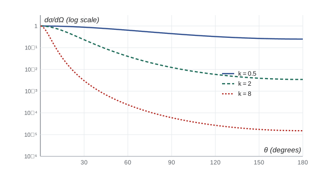
  k = 0.5: dsigma/dOmega at 10, 45, 90, 180 deg = 0.9850, 0.7608, 0.4444, 0.2500   total 6.2832 (formula 6.2832)
  k = 2.0: dsigma/dOmega at 10, 45, 90, 180 deg = 0.7950, 0.0895, 0.0123, 0.0035   total 0.7392 (formula 0.7392)
  k = 8.0: dsigma/dOmega at 10, 45, 90, 180 deg = 0.1153, 0.0007, 0.0001, 0.0000   total 0.0489 (formula 0.0489)
  Rutherford limit at 30 deg: Born with mu = 1e-6 0.87051   beta^2 / (16 E^2 sin^4) 0.87051
  Rutherford limit at 90 deg: Born with mu = 1e-6 0.01562   beta^2 / (16 E^2 sin^4) 0.01563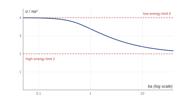

The Born approximation

When the potential is weak or the energy high, there is a more direct route. Write the Schrödinger equation as \((\nabla^2 + k^2)\psi = (2m/\hbar^2)V\psi\) and solve it with the Green's function of the left side, which turns it into an integral equation:

This is exact, but \(\psi\) appears on both sides. If the scattered wave is small compared with the incident wave inside the potential, replace \(\psi(\mathbf r')\) on the right by the plane wave. Expanding for \(r \gg r'\) then gives the first Born approximation, due to Max Born in the same 1926 paper that introduced the probability interpretation:

where \(\hbar\mathbf q = \hbar(\mathbf k' - \mathbf k)\) is the momentum transferred to the particle, \(q = 2k\sin(\theta/2)\), and the second form holds for spherical potentials. The scattering amplitude is the Fourier transform of the potential evaluated at the momentum transfer. Large momentum transfers probe small distances, which is why physicists build higher-energy accelerators to see finer structure. The same result follows from Fermi's golden rule of lesson 10, with plane-wave initial and final states and the density of states of the outgoing particle; the cross-section is the transition rate divided by the incident flux.

Yukawa and Rutherford

Hideki Yukawa proposed in 1935 that the nuclear force is carried by a massive particle, which gives a potential \(V(r) = -\beta e^{-\mu r}/r\) with range \(1/\mu\) set by the particle's mass. Its Born amplitude is

At low energy, \(k \ll \mu\), the scattering is nearly isotropic; at high energy it is concentrated in a forward cone of angle roughly \(\mu/k\), as the program's table shows. Letting \(\mu \to 0\) and replacing \(-\beta\) by \(Z_1Z_2e^2/4\pi\varepsilon_0\) turns the Yukawa potential into the Coulomb potential between two charges; the sign does not matter because only \(|f|^2\) is measured. With \(E = \hbar^2k^2/2m\), the cross-section becomes

the Rutherford formula, which Rutherford had derived in 1911 from classical orbits. By a happy accident, the exact quantum result, the first Born approximation and the classical calculation all agree for the pure Coulomb potential. Had they not, the nuclear model of the atom might have been delayed until quantum mechanics existed. The total Coulomb cross-section is infinite because the long-range potential deflects particles at every impact parameter; in real atoms the electrons screen the nucleus, which the Yukawa form models with \(1/\mu\) about the size of the atom.

Validity and form factors

The Born approximation requires the scattered wave to be small inside the potential. For a potential of depth \(V_0\) and range \(a\), that means \(V_0 \ll \hbar^2/ma^2\) at low energy, or \(V_0 \ll \hbar^2k/ma\) at high energy: fast particles spend too little time in the potential to be strongly deflected. When it applies, the Fourier-transform form gives a powerful way to measure structure. For a beam scattered by an extended charge distribution \(\rho(\mathbf r)\), the cross-section is the point-charge cross-section multiplied by \(|F(q)|^2\), where the form factor \(F(q) = \int\rho(\mathbf r)e^{-i\mathbf q\cdot\mathbf r}d^3r\) is the Fourier transform of the charge density. Robert Hofstadter measured nuclear and proton form factors this way at Stanford, finding the proton's charge radius of about 0.8 fm, and received the 1961 Nobel Prize.