Time-dependent perturbation theory: transitions, Fermi's golden rule and selection rules

Stationary states do not change. An atom in an exact eigenstate of its Hamiltonian stays there forever, with only its overall phase turning. Yet atoms absorb and emit light, nuclei decay, and molecules are excited by collisions. All of these are transitions between stationary states, caused by a perturbation that depends on time, such as the oscillating electric field of a light wave. This lesson develops the theory of such transitions. It leads to an exact solution for a two-level system driven at resonance, the Rabi oscillation; to Fermi's golden rule, the formula for a transition rate into a continuum of final states; and to the selection rules that determine which spectral lines appear.

Transition amplitudes

Let \(H = H^0 + H'(t)\), where \(H^0\) has stationary states \(\psi_n\) with energies \(E_n\). Expand the state in these, keeping the time dependence that \(H^0\) alone would produce, so that the coefficients change only because of \(H'\):

These equations are exact; \(|c_m(t)|^2\) is the probability of finding the system in state \(m\). If the system starts in state \(i\), so that \(c_i(0) = 1\), and the perturbation is weak, then to first order the right-hand side can be evaluated with \(c_n = \delta_{ni}\):

The first-order transition amplitude is the time integral of the matrix element, weighted by the oscillating phase \(e^{i\omega_{fi}t}\). A perturbation that varies slowly compared with \(1/\omega_{fi}\) produces almost no transition, because the phase averages it away; the system follows adiabatically. A perturbation that oscillates near the frequency \(\omega_{fi}\) is in resonance and produces large transition probabilities.

The two-level system: Rabi oscillations

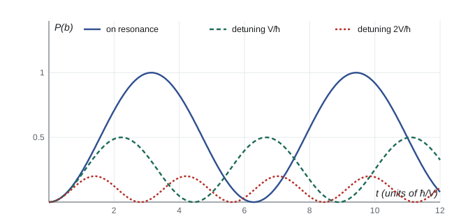
Consider two states \(a\) and \(b\), with \(E_b - E_a = \hbar\omega_0\), driven by \(H' = V\cos\omega t\) with off-diagonal matrix element \(V_{ab} = V_{ba} = V\). Each equation for \(\dot c\) then contains terms oscillating as \(e^{i(\omega_0 - \omega)t}\) and \(e^{i(\omega_0 + \omega)t}\). Near resonance, \(\omega \approx \omega_0\), the second set oscillates rapidly and averages to nearly zero; dropping it is the rotating-wave approximation. The remaining equations have constant coefficients and can be solved exactly, without assuming the perturbation is weak:

At exact resonance the system oscillates completely between \(a\) and \(b\) at the Rabi frequency \(\Omega = V/\hbar\), named for Isidor Rabi, who used such oscillations in 1938 to measure nuclear magnetic moments in molecular beams and received the Nobel Prize in 1944. A pulse of duration \(\pi/\Omega\), a \(\pi\) pulse, transfers the system completely from \(a\) to \(b\); a \(\pi/2\) pulse makes an equal superposition. Away from resonance the oscillation is faster but incomplete, with maximum probability \((V/\hbar\Omega)^2\). For short times the formula reduces to first-order perturbation theory, \(P \approx (Vt/2\hbar)^2\) at resonance. The program integrates the exact equations, counter-rotating terms included, and compares them with the Rabi formula.

Transitions into a continuum: Fermi's golden rule

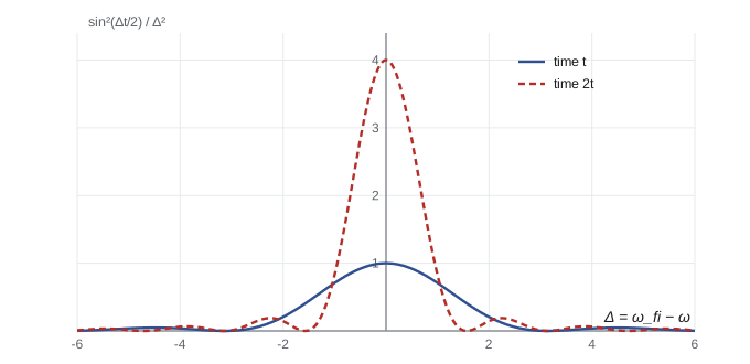
For a weak perturbation that is switched on at \(t = 0\) and oscillates at frequency \(\omega\), the first-order amplitude near resonance gives

a function of the detuning that is sharply peaked at resonance, with height proportional to \(t^2\) and width proportional to \(1/t\). For a single final state this just describes the start of a Rabi oscillation. But in most real transitions the final state belongs to a continuum: a photon emitted in any direction, an electron ejected with any momentum, a neutron scattered into any angle. Then we must sum over final states, using the density of states \(\rho(E_f)\), the number of final states per unit energy. For large \(t\) the peaked function behaves like a delta function, because \(\int\sin^2(xt/2)/x^2\,dx = \pi t/2\), and the total probability grows linearly in time. The transition rate is therefore constant:

This is Fermi's golden rule. Paul Dirac derived it in 1927, but Enrico Fermi called it golden rule number two in lectures published in 1950, and the name stuck. It is the workhorse of quantum physics: it gives the rates of atomic and nuclear transitions, of beta decay (Fermi's own application, 1934), of the absorption of light in semiconductors, and of scattering in the Born approximation of lesson 11. A constant rate implies exponential decay of the initial state, \(P_i(t) = e^{-\Gamma t}\), as the second part of the program confirms: a single level coupled weakly to 301 closely spaced levels decays exponentially at the golden-rule rate.

Emission and absorption of light

For an atom in a light wave with electric field \(\mathbf E_0\cos\omega t\), the perturbation is \(H' = -\mathbf d\cdot\mathbf E_0\cos\omega t\), where \(\mathbf d = -e\mathbf r\) is the electric dipole moment operator. This form assumes the wavelength is much larger than the atom, true for visible light, which has \(\lambda \approx 500\) nm against an atomic size of 0.1 nm. The matrix element is proportional to \(\langle f|\mathbf r|i\rangle\). Integrating the golden rule over the spectrum of incoherent light gives Einstein's rates for absorption and stimulated emission (1917). Spontaneous emission, which occurs even with no light present, cannot be derived without quantizing the electromagnetic field, but Einstein's thermodynamic argument fixes its rate:

For the hydrogen \(2p \to 1s\) transition, the Lyman alpha line, the matrix element is \(|\langle 100|z|210\rangle| = 0.745a\), and the program finds \(A = 6.26 \times 10^8\) per second, a lifetime of 1.60 ns, in agreement with measurement. The \(\omega^3\) factor explains why visible and ultraviolet transitions are fast while microwave and radio transitions, such as the 21 cm line, are slow.

import cmath, math

# 1. Rabi oscillation: two levels driven by V cos(w t); integrate the exact equations (no rotating-wave approximation)
def rabi_numeric(V, w0, w, tmax, steps=40000):
    """Amplitudes ca, cb in the interaction picture, hbar = 1. Returns P_b at tmax by RK4."""
    def deriv(t, y):
        ca, cb = y
        f = V * math.cos(w * t)
        return (-1j * f * cmath.exp(-1j * w0 * t) * cb, -1j * f * cmath.exp(1j * w0 * t) * ca)
    y = (1 + 0j, 0j); t = 0.0; h = tmax / steps
    for _ in range(steps):
        k1 = deriv(t, y)
        k2 = deriv(t + h / 2, tuple(y[i] + h / 2 * k1[i] for i in range(2)))
        k3 = deriv(t + h / 2, tuple(y[i] + h / 2 * k2[i] for i in range(2)))
        k4 = deriv(t + h, tuple(y[i] + h * k3[i] for i in range(2)))
        y = tuple(y[i] + h / 6 * (k1[i] + 2 * k2[i] + 2 * k3[i] + k4[i]) for i in range(2)); t += h
    return abs(y[1]) ** 2

def rabi_formula(V, w0, w, t):
    d = w - w0; Om = math.sqrt(d * d + V * V)          # Rabi frequency with coupling V (RWA)
    return (V / Om) ** 2 * math.sin(Om * t / 2) ** 2

w0, V = 20.0, 0.4
print("Driven two-level system, w0 = 20, coupling V = 0.4 (units hbar = 1)")
print("  detuning   t        P_b numeric   P_b Rabi formula")
for d in (0.0, 0.4):
    for t in (2.0, 4.0, 7.85):
        print(f"  {d:5.2f}   {t:6.2f}     {rabi_numeric(V, w0, w0 + d, t):.4f}        {rabi_formula(V, w0, w0 + d, t):.4f}")
print()

# 2. Fermi's golden rule: one level coupled to a ladder of N levels with uniform spacing (Bixon-Jortner model)
N, spacing, g = 301, 0.01, 0.01                   # density of states rho = 1/spacing; integrate exactly
energies = [(k - N // 2) * spacing for k in range(N)]
ca = 1 + 0j; cb = [0j] * N; h = 0.02; t = 0.0; out = []
def rhs(ca, cb, t):
    phases = [cmath.exp(-1j * e * t) for e in energies]
    dca = -1j * g * sum(p.conjugate() * c for p, c in zip(phases, cb))
    dcb = [-1j * g * p * ca for p in phases]
    return dca, dcb
for step in range(1, 1501):
    k1 = rhs(ca, cb, t)
    k2 = rhs(ca + h / 2 * k1[0], [c + h / 2 * d for c, d in zip(cb, k1[1])], t + h / 2)
    k3 = rhs(ca + h / 2 * k2[0], [c + h / 2 * d for c, d in zip(cb, k2[1])], t + h / 2)
    k4 = rhs(ca + h * k3[0], [c + h * d for c, d in zip(cb, k3[1])], t + h)
    ca += h / 6 * (k1[0] + 2 * k2[0] + 2 * k3[0] + k4[0])
    cb = [c + h / 6 * (a + 2 * b + 2 * cc + d) for c, a, b, cc, d in zip(cb, k1[1], k2[1], k3[1], k4[1])]
    t += h
    if step % 300 == 0: out.append((t, abs(ca) ** 2))
Gamma = 2 * math.pi * g * g / spacing
print(f"Golden rule test: rate 2 pi |V|^2 rho = {Gamma:.4f}")
for t, p in out:
    print(f"  t = {t:5.1f}: survival {p:.4f}   exp(-Gamma t) {math.exp(-Gamma * t):.4f}")
print()

# 3. Lyman alpha: spontaneous emission rate from the 2p - 1s dipole matrix element
a0, e, hbar, eps0, c = 5.29177e-11, 1.602176634e-19, 1.054571817e-34, 8.8541878e-12, 2.99792458e8
z12 = 2 ** 7.5 / 3 ** 5 * a0                    # |<100|z|210>| = (2^8 / 3^5) a0 / sqrt(2)
omega = 10.2 * e / hbar
A = omega ** 3 * (e * z12) ** 2 / (3 * math.pi * eps0 * hbar * c ** 3)
print(f"2p -> 1s: |<z>| = {z12 / a0:.4f} a0, A = {A:.3e} per second, lifetime {1e9 / A:.2f} ns")

Driven two-level system, w0 = 20, coupling V = 0.4 (units hbar = 1)
  detuning   t        P_b numeric   P_b Rabi formula
   0.00     2.00     0.1481        0.1516
   0.00     4.00     0.5157        0.5146
   0.00     7.85     1.0000        1.0000
   0.40     2.00     0.1406        0.1436
   0.40     4.00     0.4020        0.4095
   0.40     7.85     0.3156        0.3171

Golden rule test: rate 2 pi |V|^2 rho = 0.0628
  t =   6.0: survival 0.7023   exp(-Gamma t) 0.6859
  t =  12.0: survival 0.4775   exp(-Gamma t) 0.4705
  t =  18.0: survival 0.3270   exp(-Gamma t) 0.3227
  t =  24.0: survival 0.2224   exp(-Gamma t) 0.2214
  t =  30.0: survival 0.1523   exp(-Gamma t) 0.1518

2p -> 1s: |<z>| = 0.7449 a0, A = 6.260e+08 per second, lifetime 1.60 ns

The numerical Rabi probabilities agree with the formula to two or three decimal places; the small differences come from the counter-rotating terms the formula neglects, which shift the resonance slightly, an effect named for Felix Bloch and Arnold Siegert (1940). The decay of the coupled level follows \(e^{-\Gamma t}\) closely once the first short transient, during which the probability falls quadratically, has passed.

Selection rules

The dipole matrix element \(\langle n'\ell'm'|\mathbf r|n\ell m\rangle\) vanishes for most pairs of states, and the pattern of zeros follows from symmetry. Parity: \(\mathbf r\) is odd under inversion, and hydrogen states have parity \((-1)^\ell\), so the matrix element vanishes unless the states have opposite parity. Angular momentum: \(\mathbf r\) behaves like a vector, an object with angular momentum 1, so by the rules of lesson 3 it can change \(\ell\) by at most one, and combined with parity by exactly one. The components \(z\) and \(x \pm iy\) change \(m\) by 0 and \(\pm1\). The electric dipole selection rules are therefore

The last rule holds because \(\mathbf r\) does not act on spin, which is why singlet–triplet transitions in helium are so weak. The rules express conservation of angular momentum and parity: the photon carries one unit of angular momentum and has odd intrinsic parity. They explain why the \(2s\) state of hydrogen cannot decay by a single photon to \(1s\) (\(\Delta\ell = 0\)): it lives about 0.12 s, decaying by emitting two photons at once, compared with 1.6 ns for \(2p\). Transitions that violate the dipole rules can still occur through weaker magnetic dipole or electric quadrupole terms, or through collisions; they are called forbidden. Forbidden lines of oxygen and nitrogen dominate the spectra of thin interstellar nebulae, and forbidden lines of atomic oxygen produce the green and red light of the aurora seen over the Prairies and northern Minnesota. In such thin gases the atoms are too far apart for collisions to quench their slow decays.