Boundary value problems and the shooting method

The differential equations of lesson 5 came with all their conditions at the starting time: position and velocity now, so march forward. Many physical problems are posed differently. A cable hangs between two fixed supports; a beam is clamped at both ends; heat flows through a wall whose two faces are held at different temperatures; a quantum particle is confined to a box and its wave function must vanish at both walls. Here conditions are given at two different places, and nothing at either end tells us everything needed to start marching. These are boundary value problems. This lesson solves them by turning them into a sequence of initial value problems, the shooting method, and applies it to the most important boundary value problem in physics: finding the allowed energies of a quantum system.

Initial values versus boundary values

Consider the equation \(y'' = F(x, y, y')\) on \(a \le x \le b\). An initial value problem specifies \(y(a)\) and \(y'(a)\); under mild conditions it has exactly one solution, and the methods of lesson 5 compute it. A boundary value problem specifies, say, \(y(a) = \alpha\) and \(y(b) = \beta\). It may have exactly one solution, none, or infinitely many. The equation \(y'' = -y\) with \(y(0) = 0\) and \(y(\pi) = 0\) has the infinite family \(y = c\sin x\); with \(y(0) = 0\) and \(y(\pi) = 1\) it has no solution at all; with \(y(0) = 0\) and \(y(\pi/2) = 1\) it has the single solution \(\sin x\). The richness is not a nuisance: the cases with infinitely many solutions are precisely the eigenvalue problems that determine the modes of a vibrating string and the energy levels of an atom.

The shooting method

The idea comes from artillery. To hit a target at distance \(b\), guess a launch angle, compute where the shell lands, and adjust the angle until it lands on the target. For \(y'' = F(x, y, y')\) with \(y(a) = \alpha\), \(y(b) = \beta\), we guess the missing slope \(s = y'(a)\), integrate the initial value problem from \(a\) to \(b\), and record the miss

The boundary value problem is solved when \(m(s) = 0\), which is a root-finding problem in one variable. Lesson 3 supplies the tools: bracket the root and bisect, or use the secant method, which needs no derivative of \(m\). Each evaluation of \(m\) costs one full integration, so the number of root-finding iterations matters, and the secant method's speed is valuable.

If the equation is linear, as in \(y'' + p(x)y' + q(x)y = r(x)\), then \(y(b; s)\) depends linearly on \(s\), and two shots are enough. Integrate with slopes \(s_0\) and \(s_1\), then the slope \(s = s_0 + (s_1 - s_0)(\beta - y_0(b))/(y_1(b) - y_0(b))\) hits the target exactly, apart from the discretization error of the integrator. For a nonlinear equation the miss is a curved function of \(s\) and several secant iterations are needed.

A nonlinear target problem

Return to the baseball of lesson 5, now with a practical question: at what angle must a ball leaving the bat at 45 m/s be hit to land 100 m away? Without drag the answer comes from \(R = v_0^2\sin 2\theta/g\); with drag there is no formula. The miss function is the range minus 100 m as a function of the angle. Like the vacuum case, it has two solutions, a low line drive and a high fly ball, and bisection on two different brackets finds both.

import math

g, k = 9.81, 0.00623                       # baseball drag constant from lesson 5

def landing(v0, deg, h=0.005):
    th = math.radians(deg)
    x, y, vx, vy = 0.0, 0.0, v0 * math.cos(th), v0 * math.sin(th)
    def f(s):
        sp = math.hypot(s[2], s[3]); return [s[2], s[3], -k * sp * s[2], -g - k * sp * s[3]]
    s = [x, y, vx, vy]
    while True:
        k1 = f(s); k2 = f([s[i] + h/2*k1[i] for i in range(4)])
        k3 = f([s[i] + h/2*k2[i] for i in range(4)]); k4 = f([s[i] + h*k3[i] for i in range(4)])
        new = [s[i] + h/6*(k1[i] + 2*k2[i] + 2*k3[i] + k4[i]) for i in range(4)]
        if new[1] < 0:
            frac = s[1] / (s[1] - new[1])
            return s[0] + frac * (new[0] - s[0])
        s = new

def shoot(target, lo, hi, v0=45.0):
    m_lo = landing(v0, lo) - target
    shots = 1
    while hi - lo > 1e-6:
        mid = (lo + hi) / 2
        m_mid = landing(v0, mid) - target; shots += 1
        if m_lo * m_mid <= 0: hi = mid
        else: lo, m_lo = mid, m_mid
    return (lo + hi) / 2, shots

for lo, hi, name in ((5, 39.8, "line drive"), (39.8, 85, "fly ball")):
    ang, n = shoot(100.0, lo, hi)
    print(f"{name:10s}: launch angle {ang:8.4f} degrees, range {landing(45.0, ang):.4f} m, "
          f"{n} trajectories")
vac = [math.degrees(0.5 * math.asin(100 * g / 45**2))]
vac.append(90 - vac[0])
print("without drag the two angles would be {:.2f} and {:.2f} degrees".format(*vac))

line drive: launch angle  26.0238 degrees, range 100.0000 m, 27 trajectories
fly ball  : launch angle  55.1473 degrees, range 100.0000 m, 27 trajectories
without drag the two angles would be 14.49 and 75.51 degrees

Eigenvalue problems: a particle in a box

The time-independent Schrödinger equation in one dimension,

is a linear second-order equation with an unknown parameter, the energy \(E\). Physically acceptable solutions must satisfy boundary conditions: vanish at the walls of a box, or decay to zero far from a potential well. For most values of \(E\) no solution satisfies them; only for special values, the eigenvalues, does one exist. Those are the allowed energy levels. Shooting adapts naturally: since the equation is linear and homogeneous, the overall scale of \(\psi\) is arbitrary, so we may fix \(\psi(a) = 0\) and \(\psi'(a) = 1\) at one end and treat \(E\) itself as the shooting parameter, adjusting it until the boundary condition at the other end is met.

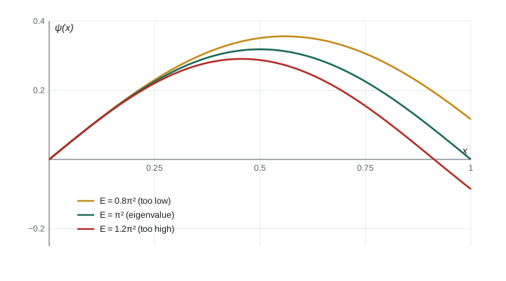
For an infinite square well of width \(L\), with \(V = 0\) inside and \(\psi(0) = \psi(L) = 0\), measure lengths in units of \(L\) and energies in units of \(\hbar^2/(2mL^2)\). The equation becomes \(\psi'' = -E\psi\) on \([0, 1]\), with exact eigenvalues \(E_n = n^2\pi^2\) and eigenfunctions \(\sin(n\pi x)\). Shooting with an energy slightly too low gives a solution that has not quite completed its half wave at \(x = 1\); slightly too high, it overshoots and crosses zero early. The eigenvalue lies where \(\psi(1)\) changes sign, and the number of interior zeros of \(\psi\) identifies which level we have found: the \(n\)th state has \(n - 1\) nodes.

The Numerov method

Equations of the form \(\psi'' = -k^2(x)\psi\), with no first-derivative term, have a special integrator that is more accurate than RK4 at the cost of only one evaluation per step. Boris Numerov devised it in the 1920s for computing the orbits of comets and the motion of the Moon. Starting from the Taylor expansions of lesson 3, \(\psi_{n+1} - 2\psi_n + \psi_{n-1} = h^2\psi_n'' + \frac{h^4}{12}\psi_n^{(4)} + O(h^6)\). Approximating \(\psi^{(4)} = (\psi'')''\) by the second difference of \(\psi'' = -k^2\psi\) and collecting terms gives

with local error \(O(h^6)\) and global error \(O(h^4)\). Two starting values are needed: \(\psi_0 = 0\) and \(\psi_1 = h\) (any small number will do, since the scale is arbitrary). For the Schrödinger equation \(k^2(x) = E - V(x)\) in the units above.

Bound states of a well and the danger of growing solutions

For a potential well that is finite in depth, the wave function in the classically forbidden region where \(V > E\) is a combination of a decaying exponential and a growing one. The physical solution keeps only the decaying part. Shooting from the left end into the right forbidden region is unstable in exactly the sense of lesson 2's recurrence: any tiny admixture of the growing solution, introduced by an energy slightly off or by rounding, is amplified exponentially, and \(\psi\) swings to \(\pm\infty\). That swing is useful, because its sign tells us whether the energy is too high or too low, so bisection on the sign of \(\psi\) at the far end still works. But the wave function itself is poor near the far end.

The robust approach shoots from both ends toward a matching point inside the well, typically the classical turning point. Each integration then runs in its stable direction, decaying into the well from the outside. The two solutions are scaled to agree at the matching point, and the eigenvalue condition is that their logarithmic derivatives \(\psi'/\psi\) agree there too. The mismatch in logarithmic derivative is a smooth function of \(E\) whose zeros are the eigenvalues.

The quantum harmonic oscillator makes an ideal test. In units where \(\hbar = m = \omega = 1\), the equation is \(\psi'' = (x^2 - 2E)\psi\), with exact energies \(E_n = n + \frac12\). The program shoots from \(x = -6\) to \(x = +6\), far enough that the true wave functions are negligible, bisects on the sign of \(\psi(6)\), and counts nodes to label the states. It also solves a finite square well, comparing with the exact energies from the matching conditions \(\sqrt{E}\tan(\sqrt{E}\,a) = \sqrt{V_0 - E}\) for even states and \(-\sqrt{E}\cot(\sqrt{E}\,a) = \sqrt{V_0 - E}\) for odd states, solved with the bisection of lesson 3. Node counting is restricted to the well and its edges, because the exponential blow-up in the forbidden region can produce spurious sign changes far from the well.

import math

def numerov_end(E, V, a, b, n=2000, window=None):
    """Integrate psi'' = (V(x) - E) psi from a to b with psi(a)=0, psi(a+h)=h.
    Return psi(b) and the number of sign changes (nodes) inside |x| < window."""
    h = (b - a) / n
    c = h * h / 12
    x0, x1 = a, a + h
    p0, p1 = 0.0, h
    k0, k1 = E - V(x0), E - V(x1)
    nodes = 0
    for i in range(1, n):
        x2 = a + (i + 1) * h
        k2 = E - V(x2)
        p2 = (2 * (1 - 5 * c * k1) * p1 - (1 + c * k0) * p0) / (1 + c * k2)
        if p2 * p1 < 0 and i < n - 1 and (window is None or abs(x2) < window):
            nodes += 1
        p0, p1, k0, k1 = p1, p2, k1, k2
        if abs(p1) > 1e200:                  # rescale; only the sign and nodes matter
            p0, p1 = p0 * 1e-200, p1 * 1e-200
    return p1, nodes

def eigen(V, a, b, Elo, Ehi, window=None):
    flo = numerov_end(Elo, V, a, b)[0]
    for _ in range(60):
        Em = (Elo + Ehi) / 2
        fm = numerov_end(Em, V, a, b)[0]
        if flo * fm <= 0: Ehi = Em
        else: Elo, flo = Em, fm
    E = (Elo + Ehi) / 2
    return E, numerov_end(E, V, a, b, window=window)[1]

print("harmonic oscillator, psi'' = (x^2 - 2E) psi; energies in units of hbar*omega")
V = lambda x: x * x                         # pass 2E as the energy argument
for n in range(5):
    E2, nodes = eigen(V, -6.0, 6.0, 2 * n + 0.5, 2 * n + 1.5)
    print(f"  state {n}: E = {E2 / 2:.10f}   exact {n + 0.5:.1f}   nodes {nodes}")

print("\ninfinite square well on [0,1], energies in units of hbar^2/(2mL^2)")
for n in (1, 2, 3):
    E, nodes = eigen(lambda x: 0.0, 0.0, 1.0, (n - 0.5)**2 * math.pi**2, (n + 0.5)**2 * math.pi**2)
    print(f"  state {n}: E = {E:.8f}   exact n^2 pi^2 = {n * n * math.pi**2:.8f}   nodes {nodes}")

V0, a_half = 50.0, 1.0                      # V = 0 for |x| < 1 and V = 50 outside
def well(x):                                # the average value is used exactly at the walls,
    d = abs(x) - a_half                     # which keeps Numerov accurate at the jump
    return 0.0 if d < -1e-9 else (V0 if d > 1e-9 else V0 / 2)
print("\nfinite square well, depth 50, half-width 1 (shooting from -5 to 5)")
found = []
E = 0.25
prev = numerov_end(E, well, -5.0, 5.0)[0]
while E < V0:
    E2 = E + 0.25
    cur = numerov_end(E2, well, -5.0, 5.0)[0]
    if prev * cur < 0:
        found.append(eigen(well, -5.0, 5.0, E, E2, window=1.5))
    E, prev = E2, cur
def even_eq(E): return math.sqrt(E) * math.sin(math.sqrt(E) * a_half) - math.sqrt(V0 - E) * math.cos(math.sqrt(E) * a_half)
def odd_eq(E):  return math.sqrt(E) * math.cos(math.sqrt(E) * a_half) + math.sqrt(V0 - E) * math.sin(math.sqrt(E) * a_half)
for E, nodes in found:
    eq = even_eq if nodes % 2 == 0 else odd_eq
    lo, hi = E - 0.05, E + 0.05
    for _ in range(60):
        mid = (lo + hi) / 2
        if eq(lo) * eq(mid) <= 0: hi = mid
        else: lo = mid
    kind = "even" if nodes % 2 == 0 else "odd "
    print(f"  E = {E:.6f}   nodes {nodes} ({kind})   transcendental equation gives {lo:.6f}")

harmonic oscillator, psi'' = (x^2 - 2E) psi; energies in units of hbar*omega
  state 0: E = 0.5000000000   exact 0.5   nodes 0
  state 1: E = 1.5000000000   exact 1.5   nodes 1
  state 2: E = 2.4999999999   exact 2.5   nodes 2
  state 3: E = 3.4999999998   exact 3.5   nodes 3
  state 4: E = 4.5000000006   exact 4.5   nodes 4

infinite square well on [0,1], energies in units of hbar^2/(2mL^2)
  state 1: E = 9.86960440   exact n^2 pi^2 = 9.86960440   nodes 0
  state 2: E = 39.47841760   exact n^2 pi^2 = 39.47841760   nodes 1
  state 3: E = 88.82643961   exact n^2 pi^2 = 88.82643961   nodes 2

finite square well, depth 50, half-width 1 (shooting from -5 to 5)
  E = 1.890949   nodes 0 (even)   transcendental equation gives 1.890854
  E = 7.525449   nodes 1 (odd )   transcendental equation gives 7.525096
  E = 16.767890   nodes 2 (even)   transcendental equation gives 16.767208
  E = 29.286793   nodes 3 (odd )   transcendental equation gives 29.285889
  E = 44.035263   nodes 4 (even)   transcendental equation gives 44.034635

The harmonic oscillator energies come out as \(0.5, 1.5, 2.5, \ldots\) to about ten digits, and the node counts \(0, 1, 2, \ldots\) label the states. The infinite well reproduces \(n^2\pi^2\). The finite well of depth 50 has five bound states, alternately even and odd, and all five agree with the roots of the exact matching conditions to about four digits. The remaining difference comes from the jump in the potential at the walls: Numerov's high order assumes a smooth \(k^2(x)\), and a discontinuity reduces it locally to second order. Placing grid points exactly on the walls and using the average potential there, as the program does, keeps the damage small; without that care the error is a hundred times larger. All of this is the same root-finding of lesson 3 with a differential equation inside the function.

Shooting versus finite differences

An alternative to shooting is to discretize the whole interval at once. Replacing \(y''\) by the three-point formula at every interior grid point turns a linear boundary value problem into a tridiagonal linear system, which lesson 8 solves in a number of operations proportional to the number of points. For an eigenvalue problem the same discretization produces a matrix eigenvalue problem, solved by the methods of lesson 9. The finite-difference approach treats both ends symmetrically and has no trouble with growing solutions, but it is limited to second order unless more elaborate formulas are used. Shooting with a high-order integrator such as Numerov's is more accurate per grid point, easy to program and natural for finding one eigenvalue at a time. Both belong in the toolbox.