Numerical integration: trapezoid, Simpson and Gaussian quadrature

Integrals are everywhere in physics: work as the integral of force, charge from charge density, the period of an oscillator from its energy, the heat capacity of a solid from its spectrum of vibrations, a probability from a wave function. Most of them cannot be done in closed form, and numerical integration, also called quadrature, replaces each by a weighted sum of function values. This lesson derives the classical rules, explains why some of them converge astonishingly fast, and shows how to handle the difficulties that real integrals throw up: singular endpoints, infinite ranges and unknown smoothness.

The trapezoid rule

Divide \([a, b]\) into \(N\) intervals of width \(h = (b - a)/N\) with points \(x_k = a + kh\). Replacing \(f\) on each interval by the straight line through its endpoint values and adding the areas of the resulting trapezoids gives

On a single interval the error of the straight-line approximation is \(-\frac{h^3}{12} f''(\xi)\), which can be shown by integrating the interpolation error \(\frac12 f''(\xi)(x - x_k)(x - x_{k+1})\). Summing \(N = (b-a)/h\) such errors gives the global error

so the composite trapezoid rule is second order. The midpoint rule, which uses the value at the centre of each interval, has error \(+\frac{(b-a)h^2}{24} f''\), half as large and of opposite sign. That relation is not a coincidence: Simpson's rule is exactly the combination \(\frac{2}{3} M + \frac{1}{3} T\) that cancels the \(h^2\) errors.

Simpson's rule

Fitting a parabola through three equally spaced points \(x_{k-1}, x_k, x_{k+1}\) and integrating it gives \(\frac{h}{3}(f_{k-1} + 4f_k + f_{k+1})\). With an even number \(N\) of intervals the composite rule is

with global error \(-\frac{(b-a)h^4}{180} f^{(4)}(\xi)\). The parabola was expected to give third order; the fourth order is a bonus from symmetry, because the rule happens to integrate cubics exactly as well. Thomas Simpson published the rule in 1743, though Johannes Kepler had used a similar barrel rule more than a century earlier. Rules of this family, built on polynomial interpolation at equally spaced points, are the Newton–Cotes formulas, published by Roger Cotes's editors in 1722. High-order Newton–Cotes rules are rarely used because their weights become large and of mixed sign, which amplifies rounding errors.

Romberg integration

The Euler–Maclaurin formula, found independently by Leonhard Euler and Colin Maclaurin in the 1730s, says that for smooth \(f\) the trapezoid error has an expansion in even powers of \(h\),

This is exactly the situation for Richardson extrapolation from lesson 3. Computing \(T(h)\), \(T(h/2)\), \(T(h/4)\) and so on, reusing the old points each time, and then extrapolating repeatedly removes \(h^2\), \(h^4\), \(h^6\) in turn. Werner Romberg proposed this systematic scheme in 1955. The first extrapolation \((4T(h/2) - T(h))/3\) is precisely Simpson's rule.

The Euler–Maclaurin formula also explains a surprise. If \(f\) is smooth and periodic and we integrate over a whole period, every coefficient \(c_{2j}\) vanishes, because the derivatives at the two ends are equal. The trapezoid rule then converges faster than any power of \(h\), typically exponentially. For a periodic integrand the humble trapezoid rule beats Simpson's rule and is the method of choice. This is why it is used to compute Fourier coefficients and why the discrete Fourier transform of lesson 11 is so accurate.

Gaussian quadrature

Newton–Cotes rules fix the points and choose the weights. Carl Friedrich Gauss asked in 1814 what happens if the points are chosen too. An \(n\)-point rule \(\sum w_i f(x_i)\) has \(2n\) free parameters, so we might hope to integrate all polynomials up to degree \(2n - 1\) exactly. On \([-1, 1]\) this is achieved by taking the \(x_i\) to be the zeros of the Legendre polynomial \(P_n\), with weights

The proof is short. Let \(p\) have degree at most \(2n - 1\) and divide it by \(P_n\): \(p = q P_n + r\) with \(q\) and \(r\) of degree at most \(n - 1\). The integral of \(q P_n\) vanishes because \(P_n\) is orthogonal to every polynomial of lower degree, and the rule gives zero for \(qP_n\) too, because \(P_n(x_i) = 0\). So the rule is exact for \(p\) if and only if it is exact for \(r\), and any \(n\)-point rule with distinct points can be made exact for polynomials of degree \(n - 1\) by choosing the weights as the integrals of the Lagrange basis polynomials. Carl Jacobi gave this orthogonal-polynomial explanation in 1826.

The nodes can be computed with tools we already have. The Legendre polynomials satisfy the three-term recurrence \((k+1)P_{k+1}(x) = (2k+1)xP_k(x) - kP_{k-1}(x)\) with \(P_0 = 1\), \(P_1 = x\), and the derivative follows from \((1 - x^2)P_n'(x) = n\,[P_{n-1}(x) - xP_n(x)]\). Starting Newton's method from \(\cos(\pi(i - 0.25)/(n + 0.5))\) converges to the \(i\)th zero in a few steps. For an interval \([a, b]\) we map \(x \mapsto \frac{a+b}{2} + \frac{b-a}{2}x\) and multiply the weights by \(\frac{b-a}{2}\). In 1969 Gene Golub and John Welsch showed that the nodes are also the eigenvalues of a symmetric tridiagonal matrix, a connection to the eigenvalue methods of lesson 9.

For smooth integrands Gauss–Legendre quadrature is spectacularly efficient: the error falls roughly exponentially with \(n\). Ten points often give twelve digits. Its weakness is that the points for different \(n\) do not overlap, so error estimates require extra work, and that it relies on smoothness: an integrand with a kink or a singularity spoils the high order.

import math

def trapezoid(f, a, b, N):
    h = (b - a) / N
    return h * (0.5 * f(a) + sum(f(a + k * h) for k in range(1, N)) + 0.5 * f(b))

def simpson(f, a, b, N):            # N even
    h = (b - a) / N
    s = f(a) + f(b) + sum((4 if k % 2 else 2) * f(a + k * h) for k in range(1, N))
    return s * h / 3

def legendre(n, x):
    """Return P_n(x) and P_n'(x) from the three-term recurrence."""
    p0, p1 = 1.0, x
    for k in range(1, n):
        p0, p1 = p1, ((2 * k + 1) * x * p1 - k * p0) / (k + 1)
    return p1, n * (p0 - x * p1) / (1 - x * x)

def gauss_nodes(n):
    nodes = []
    for i in range(1, n + 1):
        x = math.cos(math.pi * (i - 0.25) / (n + 0.5))
        for _ in range(100):
            p, dp = legendre(n, x)
            dx = p / dp
            x -= dx
            if abs(dx) < 1e-16: break
        p, dp = legendre(n, x)
        nodes.append((x, 2 / ((1 - x * x) * dp * dp)))
    return nodes

def gauss(f, a, b, n):
    c, d = (a + b) / 2, (b - a) / 2
    return d * sum(w * f(c + d * x) for x, w in gauss_nodes(n))

print("4-point Gauss-Legendre nodes and weights:")
for x, w in gauss_nodes(4):
    print(f"   x = {x:+.15f}   w = {w:.15f}")

exact = 2.0
print("\n evals   trapezoid     Simpson       Gauss")
for n in (3, 5, 9, 17, 33, 65, 129):
    et = abs(trapezoid(math.sin, 0, math.pi, n - 1) - exact)
    es = abs(simpson(math.sin, 0, math.pi, n - 1) - exact)
    eg = abs(gauss(math.sin, 0, math.pi, n) - exact) if n <= 17 else float("nan")
    print(f"{n:5d}   {et:10.2e}   {es:10.2e}   {eg:10.2e}")

# a periodic integrand: trapezoid converges exponentially
g = lambda x: 1 / (2 + math.cos(x))
exact_p = 2 * math.pi / math.sqrt(3)
print("\nperiodic integrand 1/(2 + cos x) over one period:")
for N in (4, 8, 16, 32):
    print(f"   N = {N:2d}  trapezoid error {abs(trapezoid(g, 0, 2 * math.pi, N) - exact_p):.2e}"
          f"   Simpson error {abs(simpson(g, 0, 2 * math.pi, N) - exact_p):.2e}")

4-point Gauss-Legendre nodes and weights:
   x = +0.861136311594053   w = 0.347854845137454
   x = +0.339981043584856   w = 0.652145154862546
   x = -0.339981043584856   w = 0.652145154862546
   x = -0.861136311594053   w = 0.347854845137454

 evals   trapezoid     Simpson       Gauss
    3     4.29e-01     9.44e-02     1.39e-03
    5     1.04e-01     4.56e-03     1.10e-07
    9     2.58e-02     2.69e-04     6.66e-16
   17     6.43e-03     1.66e-05     0.00e+00
   33     1.61e-03     1.03e-06          nan
   65     4.02e-04     6.45e-08          nan
  129     1.00e-04     4.03e-09          nan

periodic integrand 1/(2 + cos x) over one period:
   N =  4  trapezoid error 3.76e-02   Simpson error 1.37e-01
   N =  8  trapezoid error 1.93e-04   Simpson error 1.23e-02
   N = 16  trapezoid error 5.12e-09   Simpson error 6.43e-05
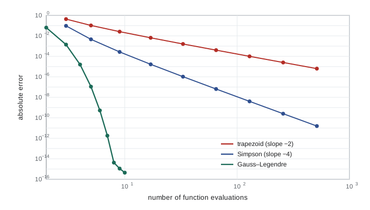
   N = 32  trapezoid error 4.44e-16   Simpson error 1.71e-09

Doubling the number of intervals divides the trapezoid error by 4 and Simpson's by 16, as their orders predict, while Gauss–Legendre reaches about \(10^{-15}\) with nine points. For the periodic integrand \(1/(2 + \cos x)\) the trapezoid rule gains more digits with every doubling of \(N\), the signature of exponential convergence, and reaches machine precision with 32 points; Simpson's rule, which weights the points unequally, does worse than the plain trapezoid rule there.

Awkward integrals

Real integrals often have features that spoil the error estimates above. An integrable singularity at an endpoint, such as \(\int_0^1 x^{-1/2}\cos x\,dx\), makes the derivatives in the error formula infinite and the convergence slow. The cure is usually a change of variable that removes it: with \(x = t^2\), \(dx = 2t\,dt\), the integral becomes \(\int_0^1 2\cos(t^2)\,dt\), which is perfectly smooth. Rules that do not evaluate at the endpoints, such as the midpoint rule and Gauss–Legendre, can at least be applied without dividing by zero.

The exact pendulum period of lesson 1 is an instructive case. Written in terms of the angle, the period is \(T = \sqrt{8L/g}\int_0^{\theta_0} d\theta/\sqrt{\cos\theta - \cos\theta_0}\), which has an inverse-square-root singularity at the turning point. The substitution \(\sin(\theta/2) = k\sin\phi\) used in lesson 1 removes it and leaves the smooth elliptic integral. Choosing good variables is often worth more than choosing a good rule.

An infinite range, such as \(\int_0^\infty e^{-x}x^3\,dx\), can be handled by truncating where the integrand is negligible, by a substitution such as \(x = t/(1-t)\) that maps \([0, \infty)\) to \([0, 1)\), or by special Gaussian rules built on other orthogonal polynomials: Gauss–Laguerre for weight \(e^{-x}\) on \([0, \infty)\) and Gauss–Hermite for weight \(e^{-x^2}\) on the whole line, the natural choice for quantum harmonic oscillator integrals.

When the integrand varies on very different scales in different places, a uniform grid wastes effort. Adaptive quadrature estimates the error on each subinterval, typically by comparing Simpson's rule on the interval with Simpson's rule on its two halves, and subdivides only where the estimate exceeds the tolerance. The difference between the two estimates is about fifteen times the error of the finer one, which supplies both an error estimate and, by Richardson, an improved value.

A physics application: the Debye heat capacity

Peter Debye explained in 1912 why the heat capacity of a solid falls to zero at low temperature. Treating the lattice vibrations as sound waves with frequencies up to a cutoff, he found the molar heat capacity

where \(R\) is the gas constant and \(\Theta_D\) the Debye temperature, about 343 K for copper. At high temperature \(C_V\) approaches the classical Dulong–Petit value \(3R \approx 24.9\) J/(mol K); at low temperature it falls as \(T^3\), the Debye law. The integrand needs care near \(x = 0\), where both numerator and denominator vanish: computing \((e^x - 1)\) with math.expm1 avoids the cancellation of lesson 2, and the limit of the integrand there is \(x^2\). The program evaluates the integral by adaptive Simpson and by Gauss–Legendre and compares with the two limits.

import math

def integrand(x):
    if x < 1e-8: return x * x                  # limit of x^4 e^x / (e^x - 1)^2
    em1 = math.expm1(x)                        # e^x - 1 without cancellation
    return x**4 * (em1 + 1) / (em1 * em1)

calls = 0
def adaptive_simpson(f, a, b, tol):
    def simp(a, fa, b, fb):
        global calls
        m = (a + b) / 2; fm = f(m); calls += 1
        return m, fm, (b - a) / 6 * (fa + 4 * fm + fb)
    def rec(a, fa, b, fb, m, fm, whole, tol, depth):
        lm, flm, left = simp(a, fa, m, fm)
        rm, frm, right = simp(m, fm, b, fb)
        if depth > 40 or abs(left + right - whole) <= 15 * tol:
            return left + right + (left + right - whole) / 15
        return (rec(a, fa, m, fm, lm, flm, left, tol / 2, depth + 1) +
                rec(m, fm, b, fb, rm, frm, right, tol / 2, depth + 1))
    fa, fb = f(a), f(b)
    m, fm, whole = simp(a, fa, b, fb)
    return rec(a, fa, b, fb, m, fm, whole, tol, 0)

def gauss20(f, a, b):
    # 20-point Gauss-Legendre nodes by Newton's method on P_20
    n, total = 20, 0.0
    c, d = (a + b) / 2, (b - a) / 2
    for i in range(1, n + 1):
        x = math.cos(math.pi * (i - 0.25) / (n + 0.5))
        for _ in range(50):
            p0, p1 = 1.0, x
            for k in range(1, n):
                p0, p1 = p1, ((2 * k + 1) * x * p1 - k * p0) / (k + 1)
            dp = n * (p0 - x * p1) / (1 - x * x)
            x -= p1 / dp
        total += 2 / ((1 - x * x) * dp * dp) * f(c + d * x)
    return d * total

R, theta_D = 8.314462618, 343.0              # copper
print("  T (K)    C_V adaptive   C_V Gauss20   T^3 law     calls")
for T in (5, 10, 20, 50, 100, 200, 300, 1000):
    calls = 0
    ia = adaptive_simpson(integrand, 0.0, theta_D / T, 1e-10)
    ig = gauss20(integrand, 0.0, theta_D / T)
    pre = 9 * R * (T / theta_D) ** 3
    low = 12 * math.pi**4 / 5 * R * (T / theta_D) ** 3
    print(f"{T:6d}   {pre * ia:12.6f}   {pre * ig:11.6f}   {low:9.6f}   {calls:5d}")
print(f"Dulong-Petit limit 3R = {3 * R:.4f} J/(mol K)")

  T (K)    C_V adaptive   C_V Gauss20   T^3 law     calls
     5       0.006021      0.006021    0.006021    3779
    10       0.048168      0.048168    0.048168    3047
    20       0.385289      0.385289    0.385347    2331
    50       4.984711      4.984711    6.021055    1103
   100      14.766135     14.766135   48.168437     499
   200      21.628251     21.628251   385.347499     227
   300      23.386227     23.386227   1300.547808     127
  1000      24.797274     24.797274   48168.437348      31
Dulong-Petit limit 3R = 24.9434 J/(mol K)

At 5 K and 10 K the heat capacity follows the \(T^3\) law, \(C_V = \frac{12\pi^4}{5} R (T/\Theta_D)^3\), which comes from extending the integral to infinity, where it equals \(4\pi^4/15\). At room temperature copper's heat capacity is already within about 6% of the Dulong–Petit value, and at 1000 K within 1%. Gauss–Legendre with only twenty function values agrees with the adaptive rule to every digit printed at every temperature, while the adaptive rule needed several thousand evaluations at the lowest temperatures, where the interval is long and its tolerance is absolute. For a smooth integrand of known shape, Gaussian quadrature is hard to beat. Adaptive rules earn their keep when the integrand has sharp features at unknown places, such as a resonance peak or a kink, which is why they are the default in general-purpose software.

Integrals in many dimensions

A product rule with \(n\) points in each of \(d\) dimensions needs \(n^d\) function values. For a three-dimensional integral with 20 points per axis that is 8000 evaluations, which is fine; for the 3N-dimensional configuration integrals of statistical mechanics it is hopeless even for a handful of particles. The error of a rule of order \(p\) with \(M\) total points behaves like \(M^{-p/d}\), so the advantage of high order evaporates as \(d\) grows. This curse of dimensionality is the reason Monte Carlo integration, whose error falls like \(M^{-1/2}\) in any dimension, takes over in lesson 10.