Numerical differentiation and root finding

Two of the most common numerical tasks in physics are finding the rate of change of a quantity known only at discrete points and finding where a function equals zero. Velocity from a table of positions, force from a computed potential, the electric field from a potential on a grid: these are derivatives. The energy of a bound state, the time a projectile lands, the eccentric anomaly of a planet at a given date, the wavelength at which a blackbody glows brightest: these are roots. This lesson builds both tools from Taylor's theorem, works out exactly how accurate they are, and shows how truncation and round-off compete.

Difference formulas from Taylor series

If \(f\) is smooth, Taylor's theorem expands it about \(x\):

Solving the plus expansion for \(f'(x)\) gives the forward difference

for some \(\xi\) between \(x\) and \(x + h\). The error term is proportional to \(h\), so the forward difference is first order. Subtracting the minus expansion from the plus expansion cancels the even powers and gives the central difference

which is second order. Adding the two expansions instead cancels the odd powers and gives the standard formula for the second derivative,

also second order. This three-point formula appears everywhere in computational physics: in the Verlet integrator of lesson 6, the shooting method of lesson 7 and the heat and wave equations of lesson 8. Using more points cancels more terms. The five-point formula

has error \(\frac{h^4}{30} f^{(5)}(\xi)\) and is fourth order. The coefficients come from requiring that the combination reproduce the derivative exactly for every polynomial up to degree four.

The competition between truncation and round-off

The error analysis above assumes exact arithmetic. In floating point, \(f(x+h)\) and \(f(x)\) each carry a rounding error of about \(\varepsilon |f|\), where \(\varepsilon \approx 10^{-16}\), and their difference, divided by \(h\), carries an error of about \(2\varepsilon|f|/h\). For the forward difference the total error is roughly

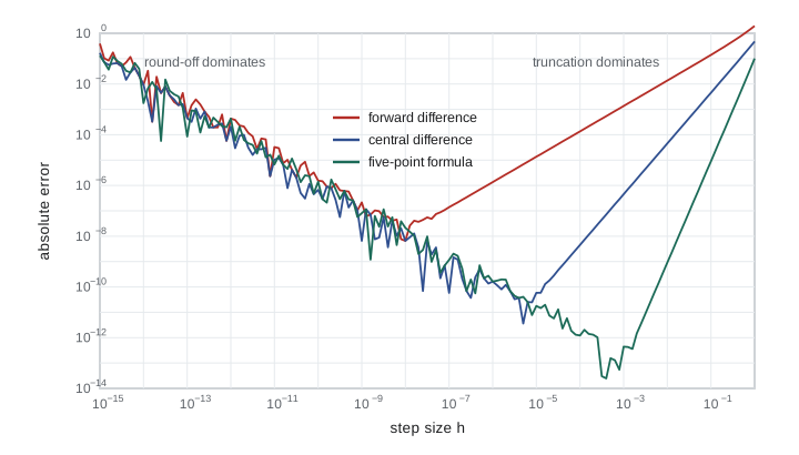
The first term falls as \(h\) shrinks and the second rises. The sum is smallest where the two are comparable, at \(h^* = 2\sqrt{\varepsilon |f|/|f''|}\). When \(f\) and \(f''\) are of similar size this is \(h^* \approx 2 \times 10^{-8}\), and the best attainable error is about \(2\sqrt{\varepsilon} \approx 3 \times 10^{-8}\): half the digits of double precision are lost no matter what. For the central difference the truncation term is \(\frac{h^2}{6}|f'''|\) and the round-off term \(\varepsilon|f|/h\), so the optimum is near \(h^* = (3\varepsilon|f|/|f'''|)^{1/3} \approx 7 \times 10^{-6}\), with error about \(\varepsilon^{2/3} \approx 4 \times 10^{-11}\). Higher-order formulas push the optimal error lower still. On a log-log plot, error against step size forms a characteristic V whose left arm has slope \(-1\) and whose right arm has slope equal to the order of the method.

import math

f, x, exact = math.exp, 1.0, math.exp(1.0)
def fwd(h): return (f(x + h) - f(x)) / h
def cen(h): return (f(x + h) - f(x - h)) / (2 * h)
def five(h): return (-f(x + 2*h) + 8*f(x + h) - 8*f(x - h) + f(x - 2*h)) / (12 * h)

print("    h        forward      central      five-point")
best = {}
for k in range(1, 15):
    h = 10.0 ** -k
    row = []
    for name, rule in (("fwd", fwd), ("cen", cen), ("five", five)):
        e = abs(rule(h) - exact)
        row.append(e)
        if e < best.get(name, (1.0, 0))[0]:
            best[name] = (e, h)
    print(f"{h:8.0e}   " + "   ".join(f"{e:10.2e}" for e in row))
for name, (e, h) in best.items():
    print(f"best {name:4s}: error {e:.1e} at h = {h:.0e}")

# Richardson extrapolation: combine central differences at h and h/2
h = 0.1
D1, D2 = cen(h), cen(h / 2)
R = (4 * D2 - D1) / 3
print(f"\ncentral h=0.1 error {abs(D1-exact):.2e}, h=0.05 error {abs(D2-exact):.2e}, "
      f"Richardson error {abs(R-exact):.2e}")

    h        forward      central      five-point
   1e-01     1.41e-01     4.53e-03     9.07e-06
   1e-02     1.36e-02     4.53e-05     9.06e-10
   1e-03     1.36e-03     4.53e-07     4.40e-13
   1e-04     1.36e-04     4.53e-09     1.23e-12
   1e-05     1.36e-05     5.86e-11     1.79e-11
   1e-06     1.36e-06     1.63e-10     1.63e-10
   1e-07     1.40e-07     5.86e-11     1.17e-09
   1e-08     6.60e-09     6.60e-09     2.14e-08
   1e-09     2.15e-07     6.60e-09     8.06e-08
   1e-10     1.55e-06     6.73e-07     1.41e-06
   1e-11     3.26e-05     1.04e-05     6.73e-06
   1e-12     4.32e-04     2.10e-04     4.32e-04
   1e-13     4.56e-04     4.56e-04     8.58e-05
   1e-14     9.34e-03     9.34e-03     1.76e-03
best fwd : error 6.6e-09 at h = 1e-08
best cen : error 5.9e-11 at h = 1e-05
best five: error 4.4e-13 at h = 1e-03

central h=0.1 error 4.53e-03, h=0.05 error 1.13e-03, Richardson error 5.66e-07

The table confirms the theory: the forward difference bottoms out near \(h = 10^{-8}\), the central difference near \(10^{-5}\) and the five-point formula near \(10^{-3}\), each with a smaller minimum error than the last. Taking \(h\) smaller than the optimum makes every formula worse.

Richardson extrapolation

If a quantity \(D(h)\) approximates \(D\) with an error expansion \(D(h) = D + c_2 h^2 + c_4 h^4 + \cdots\), as the central difference does, then

eliminates the \(h^2\) term. Lewis Fry Richardson, a pioneer of numerical weather prediction, described this deferred approach to the limit in 1911 and developed it further in 1927. The idea can be repeated to remove \(h^4\), then \(h^6\), and so on, and it applies to any method with a known error expansion: Romberg integration in lesson 4 is Richardson extrapolation of the trapezoid rule. In the program above a single extrapolation step reduced the error of the central difference at \(h = 0.05\) by a factor of more than a thousand.

For data rather than formulas, the same formulas apply to tabulated values with spacing \(h\), but now the round-off term is replaced by measurement noise, which is usually far larger than \(10^{-16}\). Differentiating noisy data amplifies the noise by about \(1/h\) for a first derivative and \(1/h^2\) for a second. Smoothing or fitting the data first, as in lesson 11, is usually wiser than differencing it directly.

Root finding by bisection

Now suppose we want \(x\) with \(f(x) = 0\). If \(f\) is continuous and \(f(a)\) and \(f(b)\) have opposite signs, the intermediate value theorem, proved by Bernard Bolzano in 1817, guarantees a root between \(a\) and \(b\). Bisection evaluates \(f\) at the midpoint \(m = (a+b)/2\) and keeps whichever half still has a sign change. Each step halves the bracket, so after \(n\) steps the root is known to within \((b - a)/2^n\). Reaching double precision from a bracket of width 1 takes about 52 steps. Bisection is slow but never fails, needs no derivative, and is the right method when reliability matters more than speed.

Newton's method

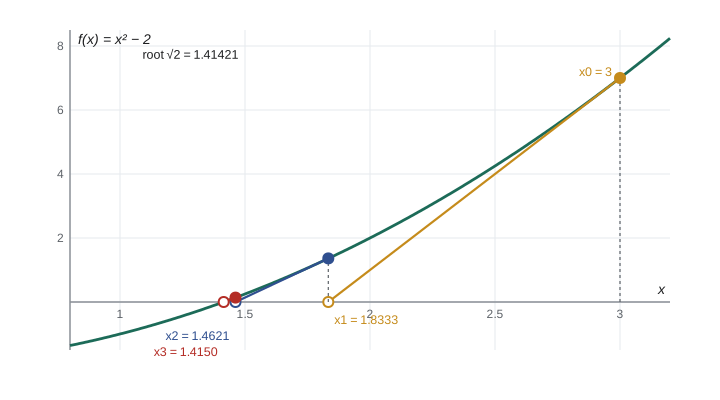
Newton's method replaces \(f\) near the current guess \(x_n\) by its tangent line and takes the tangent's zero as the next guess:

Isaac Newton described a version of the method around 1669 and Joseph Raphson published the general iteration in 1690. Its convergence near a simple root \(r\) is quadratic. To see why, expand \(f(r) = 0\) about \(x_n\): \(0 = f(x_n) + f'(x_n)(r - x_n) + \frac12 f''(\xi)(r - x_n)^2\). Dividing by \(f'(x_n)\) and using the definition of \(x_{n+1}\) gives

so the error is squared at each step and the number of correct digits roughly doubles. Five or six iterations from a good guess reach full precision. The price is that Newton's method needs the derivative and may diverge or cycle from a poor starting point, for instance near a point where \(f' = 0\). A robust strategy combines the two methods: keep a bisection bracket and take a Newton step only when it lands inside the bracket.

The secant method and fixed-point iteration

When the derivative is unavailable or expensive, the secant method replaces it by the slope through the last two iterates:

Its order of convergence is the golden ratio \((1 + \sqrt5)/2 \approx 1.618\): slower per step than Newton, but each step needs only one new function value, so it is often faster in practice.

Many equations come naturally in the form \(x = g(x)\), and the simplest approach is to iterate \(x_{n+1} = g(x_n)\). If \(g\) maps an interval into itself and \(|g'(x)| \le k < 1\) there, the iteration converges to the unique fixed point, and the error shrinks by about \(|g'(r)|\) at each step. This is linear convergence. If \(|g'(r)| > 1\) the iteration runs away from the root, even if it starts very close.

A physics example: Wien's displacement law

Planck's law gives the spectral radiance of a blackbody at temperature \(T\) as a function of wavelength. Setting its derivative with respect to wavelength to zero and writing \(x = hc/(\lambda k_B T)\) leads to the transcendental equation

Its nonzero root \(x^* \approx 4.965\) gives Wien's displacement law \(\lambda_{\max} T = hc/(k_B x^*) \approx 2.898 \times 10^{-3}\) m K, which tells us that the Sun's surface, near 5800 K, glows brightest near 500 nm, and that the cosmic microwave background at 2.725 K peaks near 1.06 mm. Wilhelm Wien found the displacement law from thermodynamics in 1893, before Planck's 1900 formula explained it. The program solves the equation by all four methods and counts the iterations.

import math

def f(x):  return x - 5 * (1 - math.exp(-x))
def df(x): return 1 - 5 * math.exp(-x)
root = None

def bisection(a, b, tol=1e-15):
    n = 0
    while b - a > tol * abs(b):
        m = (a + b) / 2
        if f(a) * f(m) <= 0: b = m
        else: a = m
        n += 1
    return (a + b) / 2, n

def newton(x, tol=1e-15):
    for n in range(1, 50):
        step = f(x) / df(x)
        x -= step
        if abs(step) < tol * abs(x): return x, n
def secant(x0, x1, tol=1e-15):
    for n in range(1, 50):
        x2 = x1 - f(x1) * (x1 - x0) / (f(x1) - f(x0))
        if abs(x2 - x1) < tol * abs(x2): return x2, n
        x0, x1 = x1, x2
def fixed_point(x, tol=1e-15):
    for n in range(1, 200):
        xn = 5 * (1 - math.exp(-x))
        if abs(xn - x) < tol * abs(xn): return xn, n
        x = xn

for name, (r, n) in (("bisection", bisection(4.0, 6.0)), ("Newton", newton(5.0)),
                     ("secant", secant(4.0, 6.0)), ("fixed point", fixed_point(5.0))):
    print(f"{name:12s} x* = {r:.15f} after {n:3d} iterations")

x = newton(5.0)[0]
h, c, kB = 6.62607015e-34, 299792458.0, 1.380649e-23
b = h * c / (kB * x)
print(f"\nWien constant b = {b:.6e} m K")
for name, T in (("Sun's surface", 5772), ("tungsten filament", 2800), ("human skin", 306),
                ("cosmic background", 2.725)):
    print(f"{name:18s} T = {T:7.1f} K   peak wavelength = {b / T * 1e9:10.1f} nm")

print("\nNewton errors from x0 = 5 (digits double each step):")
x, r = 5.0, newton(5.0)[0]
for k in range(5):
    print(f"  step {k}: error {abs(x - r):.2e}")
    x -= f(x) / df(x)

bisection    x* = 4.965114231744275 after  49 iterations
Newton       x* = 4.965114231744277 after   4 iterations
secant       x* = 4.965114231744277 after   6 iterations
fixed point  x* = 4.965114231744277 after  10 iterations

Wien constant b = 2.897772e-03 m K
Sun's surface      T =  5772.0 K   peak wavelength =      502.0 nm
tungsten filament  T =  2800.0 K   peak wavelength =     1034.9 nm
human skin         T =   306.0 K   peak wavelength =     9469.8 nm
cosmic background  T =     2.7 K   peak wavelength =  1063402.6 nm

Newton errors from x0 = 5 (digits double each step):
  step 0: error 3.49e-02
  step 1: error 2.15e-05
  step 2: error 8.33e-12
  step 3: error 8.88e-16
  step 4: error 0.00e+00

Bisection takes 49 steps, the fixed-point iteration ten (here \(|g'(x^*)| = 5e^{-x^*} \approx 0.035\), so it converges fast for a linear method), the secant method six and Newton's method four. The error table shows Newton's quadratic convergence directly: \(3 \times 10^{-2}\), \(2 \times 10^{-5}\), \(8 \times 10^{-12}\), then the level of rounding. The physical constants are the exact values that have defined the SI units since 2019, so the computed \(b = 2.897\,77 \times 10^{-3}\) m K is limited only by the root.

Kepler's equation

A planet or comet on an elliptical orbit of eccentricity \(e\) does not move at a uniform angular rate. Kepler found in 1609 that its position at time \(t\) follows from the eccentric anomaly \(E\), defined implicitly by Kepler's equation

where \(M\) is the mean anomaly, \(P\) the period and \(t_p\) the time of closest approach. There is no closed-form solution for \(E\), and for nearly two centuries astronomers solved it by hand iteration. Newton's method with \(f(E) = E - e\sin E - M\) and \(f'(E) = 1 - e\cos E\) converges in a handful of steps for any \(e < 1\) if we start from \(E_0 = M\) for small \(e\) or \(E_0 = \pi\) for highly eccentric orbits. For Halley's comet, with \(e \approx 0.967\), the fixed-point iteration \(E \gets M + e\sin E\) converges painfully slowly near perihelion, because \(|g'| = e\cos E\) is close to 1 there, while Newton's method needs at most a few steps.