Floating point, round-off and numerical stability

Every number in a physics simulation is stored in a fixed number of bits, so almost every number is slightly wrong. Usually the errors are around one part in \(10^{16}\) and nobody notices. Occasionally a calculation magnifies them a trillionfold and returns nonsense with full confidence. This lesson explains how computers represent real numbers, how rounding errors arise and propagate, and how to arrange a calculation so that they stay small. The central distinction is between a problem that is sensitive to its inputs, which no algorithm can fix, and an algorithm that is sensitive to rounding, which a better algorithm can.

How a computer stores a real number

Python's float is an IEEE 754 double-precision number, the format used by almost every computer since the standard was adopted in 1985. A double uses 64 bits: one sign bit \(s\), eleven exponent bits encoding an integer \(e\), and fifty-two fraction bits \(f_1 f_2 \ldots f_{52}\). For normal numbers the value is

a binary version of scientific notation with an implicit leading 1. The largest double is about \(1.8 \times 10^{308}\) and the smallest normal one about \(2.2 \times 10^{-308}\). Below that come subnormal numbers, which give up the implicit 1 to extend the range gradually down to about \(5 \times 10^{-324}\). The standard also defines signed infinities, produced by overflow, and NaN, meaning not a number, produced by operations such as \(0/0\) or \(\infty - \infty\). Python itself raises an exception for float division by zero, but other operations such as math.exp(1000) or arithmetic in compiled libraries follow the standard and quietly produce these special values.

The spacing between consecutive doubles is not constant: it is proportional to the size of the numbers. Between 1 and 2 the spacing is \(2^{-52} \approx 2.22 \times 10^{-16}\), a number called machine epsilon, \(\varepsilon_{\text{mach}}\). Between 1024 and 2048 the spacing is 1024 times larger. What stays constant is the relative spacing, so doubles carry about 15 to 16 significant decimal digits at every scale. Rounding a real number to the nearest double therefore introduces a relative error of at most half the spacing, the unit round-off \(u = 2^{-53} \approx 1.11 \times 10^{-16}\).

Most decimal fractions are not exactly representable in binary, in the same way that \(1/3\) has no finite decimal expansion. The number 0.1 is stored as the nearest double, which is slightly larger than 0.1. So \(0.1 + 0.2\) is computed as \(0.30000000000000004\), and \(0.1 + 0.2 = 0.3\) is false in Python. This is not a bug in Python; it is the correct result of rounding each number to binary. The lesson for programs is never to test floating-point numbers for exact equality but to compare them within a tolerance, for example with math.isclose.

import sys, math
from fractions import Fraction

print("machine epsilon      ", sys.float_info.epsilon, "=", 2.0**-52)
print("largest double       ", sys.float_info.max)
print("smallest normal      ", sys.float_info.min)
print("smallest subnormal   ", math.nextafter(0.0, 1.0))
print("spacing near 1       ", math.ulp(1.0))
print("spacing near 1e6     ", math.ulp(1.0e6))
print("spacing near 1e16    ", math.ulp(1.0e16), "(so 1e16 + 1 == 1e16 is", 1e16 + 1 == 1e16, ")")
print()
print("0.1 is stored exactly as", Fraction(0.1))
print("which in decimal is      " + format(0.1, ".30f"))
print("0.1 + 0.2 =", 0.1 + 0.2, "  equal to 0.3?", 0.1 + 0.2 == 0.3,
      "  isclose?", math.isclose(0.1 + 0.2, 0.3))
print("exp(709) =", math.exp(709), " (close to the largest double)")
try:
    math.exp(1000)
except OverflowError as e:
    print("Python raises OverflowError:", e)
print("float('inf') - float('inf') =", float("inf") - float("inf"))

machine epsilon       2.220446049250313e-16 = 2.220446049250313e-16
largest double        1.7976931348623157e+308
smallest normal       2.2250738585072014e-308
smallest subnormal    5e-324
spacing near 1        2.220446049250313e-16
spacing near 1e6      1.1641532182693481e-10
spacing near 1e16     2.0 (so 1e16 + 1 == 1e16 is True )

0.1 is stored exactly as 3602879701896397/36028797018963968
which in decimal is      0.100000000000000005551115123126
0.1 + 0.2 = 0.30000000000000004   equal to 0.3? False   isclose? True
exp(709) = 8.218407461554972e+307  (close to the largest double)
Python raises OverflowError: math range error
float('inf') - float('inf') = nan

A model of rounding

IEEE arithmetic guarantees that each basic operation is correctly rounded: the computed result of \(x + y\), \(x - y\), \(x \times y\), \(x / y\) or \(\sqrt{x}\) is the exact result rounded to the nearest double. In symbols, writing \(\mathrm{fl}(\cdot)\) for the computed value,

This model is the foundation of error analysis. It says each operation is nearly perfect. The trouble comes from combining operations, because an error made early can be magnified by later steps. The most dramatic magnifier is subtraction of nearly equal numbers.

Catastrophic cancellation

Suppose \(a = 1.000\,000\,1\) and \(b = 1.000\,000\,0\) are each known to 16 significant digits, so each carries a relative error near \(10^{-16}\), an absolute error near \(10^{-16}\). Their difference is \(10^{-7}\), but its absolute error is still about \(10^{-16}\), so its relative error is \(10^{-9}\). Seven digits have vanished. The subtraction itself was exact; it simply exposed the errors already present in \(a\) and \(b\). This loss is called cancellation, and it is catastrophic when the inputs are themselves the results of rounding.

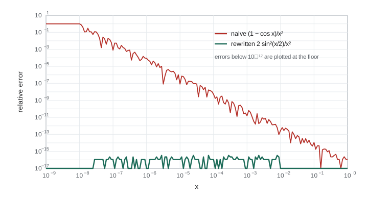
A standard example is \(f(x) = (1 - \cos x)/x^2\), which tends to \(1/2\) as \(x \to 0\). For \(x = 10^{-8}\), \(\cos x\) rounds to exactly 1, so the naive formula returns 0. The cure is to rewrite the expression so that no subtraction of nearly equal quantities occurs. The identity \(1 - \cos x = 2\sin^2(x/2)\) gives

which involves only multiplications and divisions and is accurate for every \(x\). The figure compares the relative errors of the two forms.

The quadratic formula suffers the same disease. If \(b^2 \gg 4ac\), then \(\sqrt{b^2 - 4ac} \approx |b|\), and one of the two roots \((-b \pm \sqrt{b^2 - 4ac})/(2a)\) involves the difference of nearly equal numbers. The stable approach computes the root without cancellation first,

using Vieta's relation \(x_1 x_2 = c/a\) for the second root. This matters in physics more often than one might expect, for instance when finding the time at which a fast projectile reaches a small height, or the two roots of a characteristic equation for a lightly damped circuit.

Summing many numbers

Adding a long list of numbers accumulates rounding errors, and adding a small number to a large running total loses the small number's low-order digits. Summing \(n\) numbers naively gives an error that can grow like \(n u\) times the size of the sum in the worst case, and like \(\sqrt{n}\,u\) typically. In 1965 William Kahan published compensated summation, which keeps a running correction for the digits lost at each step and achieves an error almost independent of \(n\). Python's math.fsum goes further and returns the correctly rounded sum of the inputs. When a simulation accumulates energy, time or a long Monte Carlo average, careful summation can be the difference between a clean result and a slow drift.

import math

# 1. cancellation in (1 - cos x) / x^2, whose limit is 1/2
print("    x          naive               rewritten")
for x in (1e-2, 1e-4, 1e-6, 1e-8):
    naive = (1 - math.cos(x)) / x**2
    good = 2 * math.sin(x / 2)**2 / x**2
    print(f"{x:8.0e}   {naive:.16f}   {good:.16f}")

# 2. quadratic x^2 + b x + c = 0 with b^2 >> 4c; exact small root is about -c/b
a, b, c = 1.0, 1e8, 1.0
d = math.sqrt(b * b - 4 * a * c)
naive_small = (-b + d) / (2 * a)
q = -0.5 * (b + math.copysign(d, b))
stable_small = c / q
print("\nsmall root, naive  :", naive_small)
print("small root, stable :", stable_small, " (true value -1.0000000000000000e-08)")

# 3. summing 0.1 ten million times: true answer 1,000,000
n, s, comp_s, comp_c = 10_000_000, 0.0, 0.0, 0.0
for _ in range(n):
    s += 0.1
    y = 0.1 - comp_c            # Kahan compensated summation
    t = comp_s + y
    comp_c = (t - comp_s) - y
    comp_s = t
print(f"\nnaive sum   {s:.10f}   error {s - 1e6:+.3e}")
print(f"Kahan sum   {comp_s:.10f}   error {comp_s - 1e6:+.3e}")
print(f"math.fsum   {math.fsum([0.1] * 1000):.15f}  (1000 terms, correctly rounded)")

    x          naive               rewritten
   1e-02   0.4999958333473664   0.4999958333472221
   1e-04   0.4999999969612645   0.4999999995833334
   1e-06   0.5000444502911705   0.4999999999999583
   1e-08   0.0000000000000000   0.5000000000000000

small root, naive  : -7.450580596923828e-09
small root, stable : -1e-08  (true value -1.0000000000000000e-08)

naive sum   999999.9998389754   error -1.610e-04
Kahan sum   1000000.0000000000   error +0.000e+00
math.fsum   100.000000000000000  (1000 terms, correctly rounded)

The naive formula has lost every digit by \(x = 10^{-8}\), while the rewritten one is perfect. The naive small root of the quadratic is wrong in its first digit, while the stable version is correct to full precision. The naive sum of ten million tenths drifts by about \(10^{-4}\), an error far larger than \(u\) because each addition rounds a number near \(10^6\), whose spacing is about \(10^{-10}\). The compensated sum is right to the last bit. Its only remaining error comes from 0.1 itself not being exactly representable, a data error of about \(5.6 \times 10^{-18}\) per term that totals \(5.6 \times 10^{-11}\), less than half the spacing of doubles near \(10^6\), so it disappears in the final rounding.

Conditioning: when the problem itself is sensitive

Some problems amplify input errors no matter how they are solved. The condition number measures this. For a function \(f\) of one variable, a small relative change \(\delta x/x\) in the input produces a relative change in the output of about

If \(\kappa\) is near 1, the problem is well conditioned; if it is \(10^{10}\), a relative input error of \(10^{-16}\) becomes \(10^{-6}\) in the output, and no algorithm can do better, because the input itself was only known to within rounding. For \(f(x) = x - 1\) near \(x = 1\), \(\kappa = |x/(x - 1)|\) is enormous: subtraction of nearly equal numbers is an ill-conditioned problem. For \(f(x) = \sqrt{x}\), \(\kappa = 1/2\) everywhere, a very well-conditioned problem.

Physics supplies many ill-conditioned problems. Predicting the position of a chaotic double pendulum a minute ahead is ill conditioned, because tiny changes in the starting angle grow exponentially. Inverting blurred data to recover a sharp signal is ill conditioned. In such cases the right response is not a cleverer algorithm but a different question: the statistical properties of chaotic motion, or a regularized reconstruction that accepts some blur.

Stability: when the algorithm is sensitive

An algorithm is numerically stable if it does not amplify rounding errors much beyond what the conditioning of the problem forces. The naive formula for \((1 - \cos x)/x^2\) is unstable for small \(x\) even though the problem is well conditioned there (its condition number is close to zero), and the rewritten formula is stable. A useful way to judge stability is backward error analysis, introduced by James Wilkinson in the 1950s and 1960s: an algorithm is backward stable if its computed answer is the exact answer for slightly perturbed inputs. A backward stable algorithm applied to a well-conditioned problem gives an accurate answer, and that is about all one can ask.

Recurrences are a classic source of instability. Consider the integrals \(I_n = \int_0^1 x^n e^{x-1}\,dx\). Integration by parts gives the recurrence \(I_n = 1 - n I_{n-1}\), with \(I_0 = 1 - e^{-1}\). Every \(I_n\) lies between 0 and \(1/(n+1)\), so the values shrink steadily. Run the recurrence forward and any error in \(I_0\) is multiplied by \(n\) at step \(n\), so after twenty steps it has been multiplied by \(20! \approx 2.4 \times 10^{18}\). The initial rounding error of \(10^{-17}\) becomes an error of order 10, and the computed \(I_{20}\) is wildly wrong. Run the same recurrence backward, \(I_{n-1} = (1 - I_n)/n\), and errors are divided by \(n\) at each step. Starting from the crude guess \(I_{40} = 0\), whose error is less than \(1/41\), the error has shrunk by \(40!/20! \approx 3 \times 10^{29}\) by the time we reach \(I_{20}\), which is then correct to full precision.

import math

N = 20
fwd = [1 - math.exp(-1)]
for n in range(1, N + 1):
    fwd.append(1 - n * fwd[-1])

back = {40: 0.0}                 # crude starting guess
for n in range(40, 0, -1):
    back[n - 1] = (1 - back[n]) / n

def simpson(f, a, b, m=2000):   # independent check by quadrature
    h = (b - a) / m
    s = f(a) + f(b) + sum((4 if i % 2 else 2) * f(a + i * h) for i in range(1, m))
    return s * h / 3

print(" n    forward recurrence       backward recurrence      Simpson check")
for n in (0, 5, 10, 15, 17, 18, 19, 20):
    chk = simpson(lambda x: x**n * math.exp(x - 1), 0.0, 1.0)
    print(f"{n:2d}   {fwd[n]:22.15e}   {back[n]:22.15e}   {chk:.15e}")

 n    forward recurrence       backward recurrence      Simpson check
 0    6.321205588285577e-01    6.321205588285577e-01   6.321205588285579e-01
 5    1.455329405730801e-01    1.455329405730786e-01   1.455329405731259e-01
10    8.387707005829270e-02    8.387707010339417e-02   8.387707010374869e-02
15    5.903379364190187e-02    5.901754087929777e-02   5.901754088048042e-02
17    5.719187059730757e-02    5.277111916899477e-02   5.277111917071283e-02
18   -2.945367075153627e-02    5.011985495809426e-02   5.011985496013211e-02
19    1.559619744279189e+00    4.772275579620910e-02   4.772275579860424e-02
20   -3.019239488558378e+01    4.554488407581805e-02   4.554488407861006e-02

The forward values are fine for a few steps, then go negative and explode, though every true value lies between 0 and \(1/(n+1)\). The backward values agree with an independent Simpson's rule calculation to about ten digits, the accuracy of that quadrature with 2000 intervals; lesson 4 shows how to do better. Same mathematics, opposite stability. The general principle is that a recurrence is stable in the direction in which the wanted solution grows relative to the unwanted ones. The same principle governs the shooting method of lesson 7 and the time-stepping schemes of lesson 5.

Practical defences

A short checklist covers most situations. Look for subtractions of nearly equal quantities and rewrite them using identities, series expansions or conjugates: \(\sqrt{x+1} - \sqrt{x} = 1/(\sqrt{x+1} + \sqrt{x})\). Avoid computing intermediate quantities that overflow: math.hypot computes \(\sqrt{x^2 + y^2}\) without squaring huge numbers, and log-sum-exp tricks handle sums of large exponentials in statistical mechanics. Accumulate long sums with math.fsum or compensated summation. Run recurrences in their stable direction. Use exact integers or fractions.Fraction for combinatorial quantities and Python's math.comb for binomial coefficients, which are exact. And when in doubt, repeat the calculation with a different but equivalent method and compare.

When rounding errors made the news

Several famous failures trace back to number representation. During the 1991 Gulf War a Patriot missile battery at Dhahran failed to intercept an incoming missile, and 28 soldiers were killed. The system counted time in tenths of a second in a 24-bit fixed-point register; since 0.1 is not exact in binary, the clock drifted by about a third of a second after 100 hours of continuous operation, enough to misplace the target. In 1996 the first Ariane 5 rocket destroyed itself 37 seconds after launch when a 64-bit floating-point velocity was converted to a 16-bit integer that could not hold it. And in the early 1980s the index of the Vancouver Stock Exchange, recomputed thousands of times a day and truncated rather than rounded each time, lost about half its value over less than two years through truncation alone before the error was found and corrected. The common thread is not that floating point is untrustworthy but that its limits must be respected by design.

The IEEE 754 standard owes much to William Kahan, who received the Turing Award in 1989 for his work on floating-point computation. The standard was revised in 2008, adding decimal formats and a fused multiply-add operation that computes \(xy + z\) with a single rounding, and again in 2019. Python exposes the fused operation as math.fma from version 3.13.