Monte Carlo methods: random numbers, integration and the Metropolis algorithm

Some of the most powerful methods in computational physics use randomness on purpose. Throw random points into a region and the fraction that lands inside a shape measures its area. Let a particle take random steps and its spreading reproduces diffusion. Propose random changes to a configuration of atoms and accept them with the right probability, and the configurations visited follow the Boltzmann distribution of statistical mechanics. These are Monte Carlo methods, named by Nicholas Metropolis after the casino, and developed by Stanislaw Ulam and John von Neumann at Los Alamos between 1946 and 1949 for neutron transport calculations. Their error falls only as the inverse square root of the number of samples, but that rate is the same in one dimension or a thousand, and for high-dimensional problems nothing else comes close.

Pseudorandom numbers

Computers are deterministic, so the random numbers they produce are pseudorandom: a deterministic sequence designed to pass statistical tests of randomness. The oldest family is the linear congruential generator of Derrick Lehmer from 1949,

which produces numbers \(u_k\) in \([0, 1)\). With well-chosen constants it is fast and adequate for simple uses, but its flaws can be serious. The generator RANDU, widely used on IBM computers in the 1960s and 1970s, took \(a = 65539\), \(c = 0\), \(m = 2^{31}\). Because \(a = 2^{16} + 3\), every triple of consecutive outputs satisfies \(x_{k+2} = 6x_{k+1} - 9x_k \pmod{2^{31}}\), so when plotted as points in a cube they all lie on just 15 planes. George Marsaglia showed in 1968 that all linear congruential generators share this lattice structure to some degree, and many published simulations had to be redone.

Python's random module uses the Mersenne Twister of Makoto Matsumoto and Takuji Nishimura, published in 1998, whose period is \(2^{19937} - 1\) and whose outputs are equidistributed in up to 623 dimensions. It is excellent for simulation, though not for cryptography, for which Python offers the secrets module. Every simulation should fix the seed with random.seed or, better, create its own generator with random.Random(seed), so that results can be reproduced exactly and a bug can be chased through the same sequence of numbers.

Sampling from distributions

Uniform numbers are turned into other distributions in three main ways. The inverse transform method uses the cumulative distribution \(F(x) = P(X \le x)\): if \(u\) is uniform on \((0, 1)\), then \(x = F^{-1}(u)\) has the desired distribution. For radioactive decay with mean lifetime \(\tau\), \(F(t) = 1 - e^{-t/\tau}\), so \(t = -\tau\ln(1 - u)\) samples a decay time. The Box–Muller method of George Box and Mervin Muller, from 1958, turns two uniform numbers into two independent standard normal numbers: with \(r = \sqrt{-2\ln u_1}\) and \(\theta = 2\pi u_2\), the numbers \(r\cos\theta\) and \(r\sin\theta\) are Gaussian. And von Neumann's rejection method of 1951 samples any density \(p(x)\) bounded by \(c\,g(x)\) for some easy density \(g\): draw \(x\) from \(g\) and accept it with probability \(p(x)/(c\,g(x))\), otherwise draw again. The fraction accepted is \(1/c\).

import math, random

# RANDU: consecutive triples lie on 15 planes because x[k+2] = 6 x[k+1] - 9 x[k] (mod 2^31)
m, a = 2**31, 65539
x = [1]
for _ in range(10002):
    x.append(a * x[-1] % m)
viol = sum((x[k+2] - 6 * x[k+1] + 9 * x[k]) % m != 0 for k in range(10000))
planes = {round((9 * x[k] - 6 * x[k+1] + x[k+2]) / m) for k in range(10000)}
print(f"RANDU triples violating the plane relation: {viol}; distinct planes used: {len(planes)}")

rng = random.Random(234)                         # Mersenne Twister with a fixed seed
print("first three uniforms with seed 234:", [round(rng.random(), 6) for _ in range(3)])

# inverse transform: decay times for tau = 2.2 microseconds (the muon lifetime)
tau = 2.2
times = [-tau * math.log(1 - rng.random()) for _ in range(100000)]
mean = sum(times) / len(times)
frac = sum(t > 5 for t in times) / len(times)
print(f"decay times: mean {mean:.4f} (expect {tau}), fraction surviving 5 us {frac:.4f}"
      f" (expect {math.exp(-5 / tau):.4f})")

# Box-Muller normal deviates
z = []
for _ in range(50000):
    u1, u2 = 1 - rng.random(), rng.random()
    r, th = math.sqrt(-2 * math.log(u1)), 2 * math.pi * u2
    z += [r * math.cos(th), r * math.sin(th)]
mu = sum(z) / len(z); var = sum((v - mu)**2 for v in z) / (len(z) - 1)
within = sum(abs(v) < 1 for v in z) / len(z)
print(f"Box-Muller: mean {mu:+.4f}, variance {var:.4f}, fraction within one sigma {within:.4f} (expect 0.6827)")

RANDU triples violating the plane relation: 0; distinct planes used: 15
first three uniforms with seed 234: [0.341853, 0.865595, 0.857916]
decay times: mean 2.1986 (expect 2.2), fraction surviving 5 us 0.1031 (expect 0.1030)
Box-Muller: mean -0.0008, variance 1.0016, fraction within one sigma 0.6832 (expect 0.6827)

Monte Carlo integration

To estimate \(I = \int_V f(\mathbf{x})\,d\mathbf{x}\) over a region of volume \(V\), draw \(N\) points \(\mathbf{x}_i\) uniformly in the region and average:

The estimate is a random variable. Its mean is exactly \(I\), and by the central limit theorem its distribution approaches a normal distribution with standard deviation

which can itself be estimated from the samples. The error falls like \(N^{-1/2}\): a hundred times more samples buy one more digit. That is slow compared with Simpson's rule in one dimension, whose error falls like \(N^{-4}\). But the Monte Carlo rate does not depend on the dimension, while a grid rule's error, as lesson 4 showed, falls like \(N^{-p/d}\). For \(d\) larger than about \(2p\), Monte Carlo wins, and in statistical mechanics, where \(d\) is three times the number of particles, it is the only option.

The classic first example estimates \(\pi\). Points uniform in the unit square land inside the quarter circle \(x^2 + y^2 < 1\) with probability \(\pi/4\), so four times the fraction inside estimates \(\pi\). The error behaves as \(\sqrt{\pi(4 - \pi)/N} \approx 1.64/\sqrt N\).

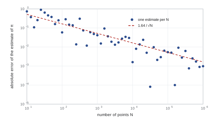
Variance reduction makes Monte Carlo more efficient. In importance sampling we draw points from a density \(p(\mathbf{x})\) that resembles \(|f|\) and average \(f/p\), which has the same mean but smaller variance if \(p\) is well chosen. An integrand with a singularity is a dramatic example. For \(\int_0^1 x^{-1/2}e^{-x}\,dx\), uniform sampling gives an estimator \(x^{-1/2}e^{-x}\) whose variance is infinite, because \(\int_0^1 x^{-1}\,dx\) diverges, so the error does not even fall as \(N^{-1/2}\). Sampling \(x = u^2\), whose density is \(p(x) = 1/(2\sqrt x)\), turns the estimator into \(2e^{-x}\), which is bounded and well behaved.

import math, random

rng = random.Random(234)

print("Monte Carlo estimates of pi")
for N in (100, 10_000, 1_000_000):
    inside = sum(rng.random()**2 + rng.random()**2 < 1 for _ in range(N))
    est = 4 * inside / N
    print(f"  N = {N:9d}: {est:.5f}   error {abs(est - math.pi):.1e}   expected size {1.64 / math.sqrt(N):.1e}")

print("\nvolume of the unit ball in d dimensions (exact pi^(d/2) / Gamma(d/2 + 1))")
N = 100_000
for d in (2, 3, 5, 8, 10):
    hits = sum(sum(rng.uniform(-1, 1)**2 for _ in range(d)) < 1 for _ in range(N))
    est, exact = 2**d * hits / N, math.pi**(d / 2) / math.gamma(d / 2 + 1)
    err = 2**d * math.sqrt(hits / N * (1 - hits / N) / N)
    print(f"  d = {d:2d}: {est:7.4f} +- {err:.4f}   exact {exact:.4f}")

print("\nintegral of exp(-x)/sqrt(x) on (0,1); exact sqrt(pi) erf(1) =", f"{math.sqrt(math.pi) * math.erf(1):.6f}")
for N in (1000, 100_000):
    plain = [math.exp(-u) / math.sqrt(u) for u in (1 - rng.random() for _ in range(N))]
    imp = [2 * math.exp(-u * u) for u in (rng.random() for _ in range(N))]
    for name, s in (("uniform sampling   ", plain), ("importance sampling", imp)):
        m = sum(s) / N; sd = math.sqrt(sum((v - m)**2 for v in s) / (N - 1))
        print(f"  N = {N:6d} {name}: {m:.6f} +- {sd / math.sqrt(N):.6f}")

Monte Carlo estimates of pi
  N =       100: 2.64000   error 5.0e-01   expected size 1.6e-01
  N =     10000: 3.15960   error 1.8e-02   expected size 1.6e-02
  N =   1000000: 3.13913   error 2.5e-03   expected size 1.6e-03

volume of the unit ball in d dimensions (exact pi^(d/2) / Gamma(d/2 + 1))
  d =  2:  3.1446 +- 0.0052   exact 3.1416
  d =  3:  4.1850 +- 0.0126   exact 4.1888
  d =  5:  5.2390 +- 0.0374   exact 5.2638
  d =  8:  3.9603 +- 0.0999   exact 4.0587
  d = 10:  2.8570 +- 0.1708   exact 2.5502

integral of exp(-x)/sqrt(x) on (0,1); exact sqrt(pi) erf(1) = 1.493648
  N =   1000 uniform sampling   : 1.508794 +- 0.060492
  N =   1000 importance sampling: 1.499866 +- 0.012628
  N = 100000 uniform sampling   : 1.492492 +- 0.010154
  N = 100000 importance sampling: 1.493499 +- 0.001269

The errors for \(\pi\) have the size that \(1.64/\sqrt N\) predicts, sometimes a little larger and sometimes smaller, as random errors should. The ball volumes agree with the exact values to within about two standard errors in every dimension, though the relative error grows with \(d\) because the ball fills an ever smaller fraction of the cube: in ten dimensions only about one point in four hundred lands inside, a hint that uniform sampling fails in very high dimensions and that sampling must concentrate where the integrand matters. For the singular integral, importance sampling gives a smaller and trustworthy error bar; the uniform estimator's quoted error is itself unreliable, because its variance is infinite.

Random walks

A particle that takes independent random steps of length \(\ell\) every \(\tau\) seconds wanders away from its start with a mean squared displacement that grows linearly in time, \(\langle x^2\rangle = 2Dt\) in each direction, with diffusion constant \(D = \ell^2/(2\tau)\). Albert Einstein derived this relation in 1905 and used it to connect the jittering Brownian motion of pollen grains with the existence of molecules, and Jean Perrin's measurements of 1908 confirmed it and yielded Avogadro's number. Random walk simulations reproduce the heat equation of lesson 8 statistically: the density of many walkers obeys \(\partial_t\rho = D\nabla^2\rho\). Monte Carlo transport codes for neutrons, photons in stellar interiors and electrons in detectors follow individual particles on such walks, with step lengths and scattering angles drawn from physical probability distributions.

Markov chains and the Metropolis algorithm

In statistical mechanics a system at temperature \(T\) is found in a configuration \(s\) with the Boltzmann probability \(\pi(s) = e^{-E(s)/k_BT}/Z\), where the partition function \(Z\) sums \(e^{-E/k_BT}\) over all configurations. Thermal averages \(\langle A\rangle = \sum_s A(s)\pi(s)\) are integrals over an enormous space, and uniform sampling is hopeless, because almost all configurations have negligible weight. We need to sample configurations in proportion to \(\pi(s)\) without knowing \(Z\).

In 1953 Nicholas Metropolis, Arianna Rosenbluth, Marshall Rosenbluth, Augusta Teller and Edward Teller published the solution. Build a Markov chain, a random walk through configuration space in which each step depends only on the current configuration. From the current \(s\), propose a trial \(s'\) by a symmetric rule, such as moving one particle by a random amount. Then accept the move with probability

and otherwise keep \(s\), counting it again. Downhill moves are always accepted, and uphill moves are accepted with the Boltzmann factor of the energy increase. The rule satisfies detailed balance, \(\pi(s)P(s \to s') = \pi(s')P(s' \to s)\), because the ratio of acceptance probabilities in the two directions is exactly \(\pi(s')/\pi(s)\). A chain that obeys detailed balance and can reach every configuration has \(\pi\) as its stationary distribution, so after an initial equilibration period the configurations it visits are distributed according to Boltzmann's law. Only energy differences appear, so \(Z\) is never needed. The paper's calculation, of the equation of state of a two-dimensional fluid of hard disks, ran on the MANIAC computer; Arianna Rosenbluth wrote the code.

Three practical points matter. The step size of the trial moves should give an acceptance rate that is neither tiny, so that the chain sticks, nor near 1, so that it barely moves; something between 20% and 60% is typical. The first part of the chain, before it has forgotten its starting point, must be discarded. And successive configurations are correlated, so the effective number of independent samples is smaller than the chain length; lesson 12 measures this with the autocorrelation time and handles it with block averages.

The program applies Metropolis sampling to a single classical particle in the quartic potential \(V(x) = x^4/4\) at \(k_BT = 1\), for which \(\langle x^2\rangle = \int x^2e^{-x^4/4}dx / \int e^{-x^4/4}dx = 2\Gamma(3/4)/\Gamma(1/4) \approx 0.6760\), and in the harmonic potential \(x^2/2\), for which equipartition gives \(\langle x^2\rangle = 1\).

import math, random

def metropolis(V, kT=1.0, step=1.5, n=200_000, burn=10_000, seed=234):
    rng = random.Random(seed)
    x, Ex = 3.0, V(3.0)                 # deliberately poor start
    acc, s1, s2 = 0, 0.0, 0.0
    for i in range(n + burn):
        xt = x + rng.uniform(-step, step)
        Et = V(xt)
        if Et <= Ex or rng.random() < math.exp(-(Et - Ex) / kT):
            x, Ex = xt, Et
            if i >= burn: acc += 1
        if i >= burn:
            s1 += x * x; s2 += (x * x) ** 2
    mean = s1 / n
    return mean, acc / n

quartic = lambda x: x**4 / 4
harmonic = lambda x: x * x / 2
exact_q = 2 * math.gamma(0.75) / math.gamma(0.25)
for name, V, exact in (("quartic  x^4/4", quartic, exact_q), ("harmonic x^2/2", harmonic, 1.0)):
    for step in (0.2, 1.5, 6.0):
        m, a = metropolis(V, step=step)
        print(f"{name}  step {step:3.1f}: <x^2> = {m:.4f} (exact {exact:.4f}), acceptance {a:.2f}")

quartic  x^4/4  step 0.2: <x^2> = 0.6834 (exact 0.6760), acceptance 0.96
quartic  x^4/4  step 1.5: <x^2> = 0.6750 (exact 0.6760), acceptance 0.71
quartic  x^4/4  step 6.0: <x^2> = 0.6814 (exact 0.6760), acceptance 0.23
harmonic x^2/2  step 0.2: <x^2> = 1.0177 (exact 1.0000), acceptance 0.96
harmonic x^2/2  step 1.5: <x^2> = 1.0015 (exact 1.0000), acceptance 0.71
harmonic x^2/2  step 6.0: <x^2> = 0.9922 (exact 1.0000), acceptance 0.27

With a moderate step the averages agree with the exact values to about two or three decimals. With a tiny step nearly every move is accepted, but the particle crawls and successive samples are highly correlated, so the estimate is noisier for the same work. With a huge step most proposals land far up the walls and are rejected, and the chain again moves slowly. The best step balances the two. Every result is a statistical estimate, and quoting it without an error bar, which must account for the correlations, is incomplete; lesson 12 shows how to compute that error bar for the Ising model.