Symplectic integrators and orbital mechanics

Lesson 5 showed that the classical Runge–Kutta method is very accurate over a short time but slowly loses energy from an oscillator. For a simulation of the solar system over a billion years, or of molecules in a liquid over millions of vibrations, that slow drift is fatal: the planets would spiral into the Sun and the liquid would freeze. This lesson introduces integrators designed around the geometry of mechanics rather than around the Taylor series. They are only second order, yet their energy errors stay bounded forever. They are the workhorses of celestial mechanics, molecular dynamics and plasma physics.

What mechanics conserves

A system without friction can be described by a Hamiltonian \(H(q, p)\), the total energy as a function of positions \(q\) and momenta \(p\), with Hamilton's equations \(\dot q = \partial H/\partial p\), \(\dot p = -\partial H/\partial q\). For a particle in a potential \(V\), \(H = p^2/2m + V(q)\), and these reduce to Newton's law. Hamiltonian flows have several conserved properties. Energy is conserved when \(H\) does not depend on time. Angular momentum is conserved when \(V\) depends only on distance. And, more subtly, the flow preserves area in phase space, a result known as Liouville's theorem: a blob of initial conditions may be stretched and folded, but its area in the \((q, p)\) plane never changes. In many dimensions the preserved structure is called the symplectic form, and a map that preserves it is symplectic.

Euler's method multiplies phase-space area by \(1 + h^2\omega^2\) per step for an oscillator, which is why its orbits spiral outward. RK4 multiplies it by slightly less than 1, which is why its orbits spiral slowly inward. A symplectic integrator is a numerical method whose step map is exactly symplectic. It cannot conserve the true energy exactly, but it turns out to conserve a nearby modified energy almost exactly, so the true energy merely oscillates within a narrow band for exponentially long times.

Symplectic Euler

Consider a small change to Euler's method: update the velocity first, then use the new velocity to update the position,

This is the symplectic Euler method, popularized for physics students by Alan Cromer in 1981 as the Euler–Cromer method after he noticed that students who made this apparent mistake got better results. For the oscillator \(a = -\omega^2 x\), the step is the linear map with matrix

whose determinant is exactly 1, so phase-space area is preserved. The orbits are ellipses slightly tilted from the true circle, closed and stable for \(h\omega < 2\). The method is still first order, but its errors no longer accumulate into a spiral.

Leapfrog and velocity Verlet

A symmetric version gains second order. Writing the second derivative with the three-point formula of lesson 3, \(x_{n+1} - 2x_n + x_{n-1} = h^2 a(x_n)\), gives the position Verlet or Störmer method

Carl Störmer used it in 1907 to compute the paths of charged particles in the Earth's magnetic field while studying the aurora, and Loup Verlet used it in 1967 in some of the first molecular dynamics simulations of liquid argon. The same method can be written with velocities as the velocity Verlet scheme, also called kick–drift–kick leapfrog:

Each step needs only one new force evaluation, since \(a(x_{n+1})\) is reused at the start of the next step. The method has four virtues that matter in physics. It is second order. It is symplectic, being a composition of a half kick, a drift and a half kick, each of which is an exact flow of part of the Hamiltonian and so preserves phase-space area. It is time reversible: running it backward with \(-h\) exactly retraces the trajectory, as the true dynamics would. And for central forces it conserves angular momentum exactly, because the kicks are along the radius vector and the drift is along the velocity, neither of which changes \(\mathbf{r} \times \mathbf{v}\).

Why does the energy stay bounded? A deep result of backward error analysis, worked out by Ernst Hairer, Christian Lubich, Gerhard Wanner and others around 2000, shows that the numerical trajectory of a symplectic method is the exact trajectory of a modified Hamiltonian \(\tilde H = H + h^2 H_2 + h^4 H_4 + \cdots\), up to errors that are exponentially small in \(1/h\). The numerical solution conserves \(\tilde H\), and since \(\tilde H\) differs from \(H\) by \(O(h^2)\), the true energy oscillates with amplitude \(O(h^2)\) but never drifts. A non-symplectic method has no such conserved quantity, and its energy error grows steadily.

The Kepler problem

A planet of negligible mass orbiting the Sun obeys \(\ddot{\mathbf{r}} = -GM\,\mathbf{r}/r^3\). Astronomical units and years make the numbers pleasant: with distances in AU and time in years, \(GM_\odot = 4\pi^2\) AU\(^3\)/yr\(^2\), and an orbit with semi-major axis 1 has period 1. The energy per unit mass is \(E = \frac12 v^2 - GM/r\), the angular momentum per unit mass is \(L = |\mathbf{r} \times \mathbf{v}|\), and for an ellipse \(E = -GM/(2a)\). Starting at perihelion distance \(r_p = a(1 - e)\) with speed \(v_p = \sqrt{GM(1 + e)/(a(1 - e))}\) gives an orbit of eccentricity \(e\).

An eccentric orbit is a demanding test, because the planet moves slowly far from the Sun and very fast near it, and the error made at each perihelion passage accumulates. The program below integrates an orbit with \(e = 0.6\) for 200 periods with three methods at equal cost: velocity Verlet and symplectic Euler with 500 steps per orbit, and RK4 with 125 steps per orbit, since RK4 needs four force evaluations per step.

import math

GM = 4 * math.pi ** 2
a_axis, ecc = 1.0, 0.6
def accel(x, y):
    r3 = (x * x + y * y) ** 1.5
    return -GM * x / r3, -GM * y / r3
def energy(x, y, vx, vy): return 0.5 * (vx*vx + vy*vy) - GM / math.hypot(x, y)
def angmom(x, y, vx, vy): return x * vy - y * vx

def start():
    rp = a_axis * (1 - ecc)
    return rp, 0.0, 0.0, math.sqrt(GM * (1 + ecc) / rp)

def verlet(n_orbits, per_orbit):
    h = 1.0 / per_orbit
    x, y, vx, vy = start(); ax, ay = accel(x, y)
    for _ in range(n_orbits * per_orbit):
        vx += 0.5 * h * ax; vy += 0.5 * h * ay
        x += h * vx; y += h * vy
        ax, ay = accel(x, y)
        vx += 0.5 * h * ax; vy += 0.5 * h * ay
    return x, y, vx, vy

def sym_euler(n_orbits, per_orbit):
    h = 1.0 / per_orbit
    x, y, vx, vy = start()
    for _ in range(n_orbits * per_orbit):
        ax, ay = accel(x, y)
        vx += h * ax; vy += h * ay
        x += h * vx; y += h * vy
    return x, y, vx, vy

def rk4(n_orbits, per_orbit):
    h = 1.0 / per_orbit
    def f(s):
        ax, ay = accel(s[0], s[1]); return [s[2], s[3], ax, ay]
    s = list(start())
    for _ in range(n_orbits * per_orbit):
        k1 = f(s); k2 = f([s[i] + h/2*k1[i] for i in range(4)])
        k3 = f([s[i] + h/2*k2[i] for i in range(4)]); k4 = f([s[i] + h*k3[i] for i in range(4)])
        s = [s[i] + h/6*(k1[i] + 2*k2[i] + 2*k3[i] + k4[i]) for i in range(4)]
    return tuple(s)

E0, L0 = energy(*start()), angmom(*start())
print(f"initial energy {E0:.6f}, exact -GM/(2a) = {-GM / 2:.6f}")
print("orbits   method            rel. energy error   rel. ang. mom. error")
for n in (10, 50, 200):
    for name, fn, per in (("velocity Verlet", verlet, 500), ("symplectic Euler", sym_euler, 500),
                          ("RK4", rk4, 125)):
        st = fn(n, per)
        dE = (energy(*st) - E0) / abs(E0); dL = (angmom(*st) - L0) / L0
        print(f"{n:6d}   {name:16s}   {dE:+16.3e}   {dL:+18.3e}")

initial energy -19.739209, exact -GM/(2a) = -19.739209
orbits   method            rel. energy error   rel. ang. mom. error
    10   velocity Verlet          +3.648e-04           +1.767e-15
    10   symplectic Euler         -2.999e-02           -1.767e-15
    10   RK4                      -6.994e-04           -7.784e-05
    50   velocity Verlet          +1.171e-03           -2.827e-15
    50   symplectic Euler         -1.902e-03           -4.064e-15
    50   RK4                      -3.518e-03           -3.889e-04
   200   velocity Verlet          +1.133e-03           -1.767e-14
   200   symplectic Euler         +7.380e-03           -2.827e-15
   200   RK4                      -1.393e-02           -1.556e-03

The results show the qualitative difference. The RK4 energy error grows steadily with the number of orbits, always in the same direction: the planet is slowly sinking toward the Sun. The Verlet energy error does not grow: sampled at whole periods it wanders around \(10^{-3}\), set by where in its oscillation the sample happens to fall, and it is no larger after 200 orbits than after 50. Its angular momentum error is at the level of rounding. Symplectic Euler, being only first order, has a larger but equally bounded energy error. Over short times RK4 is the more accurate method; over long times the symplectic methods win decisively, and the longer the simulation the larger their advantage.

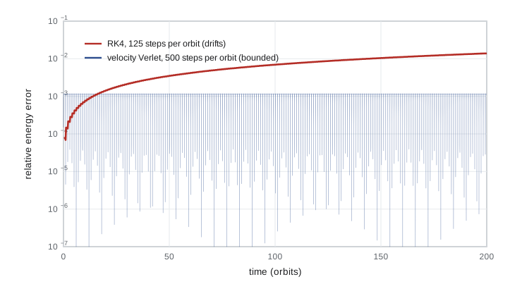
Verlet's energy error is not small at every instant: it rises sharply at each perihelion passage, where the step is coarsest relative to the motion, and falls back afterward. Its time-averaged value is set by the modified Hamiltonian. Variable time steps would reduce the spikes, but they must be introduced carefully, because a naively varied step destroys the symplectic property. Practical orbital codes either use fixed steps, regularize the equations so that a fixed step in a new time variable corresponds to small steps near the Sun, or use methods built specifically for nearly Keplerian motion, such as the Wisdom–Holman map of 1991, which splits each step into an exact Kepler orbit and a kick from the planets.

Higher order by composition

Because velocity Verlet is symmetric, it can be composed with itself to cancel error terms while staying symplectic. Haruo Yoshida showed in 1990 that three Verlet steps of sizes \(w_1h, w_0h, w_1h\), with \(w_1 = 1/(2 - 2^{1/3})\) and \(w_0 = 1 - 2w_1\), form a fourth-order symplectic method. The middle step is negative, a backward step in time, which looks strange but is harmless. Repeating the trick gives sixth and eighth order. These methods are used when long integrations need both high accuracy and bounded energy error.

Three bodies

The two-body problem is solved exactly by Kepler's ellipses; the three-body problem is generally chaotic and was the problem that led Henri Poincaré in the 1890s to discover sensitive dependence on initial conditions. A few remarkable periodic solutions exist. In 1993 Cristopher Moore found numerically that three equal masses can chase each other around a figure-eight curve, and in 2000 Alain Chenciner and Richard Montgomery proved that the orbit exists. With \(G = m = 1\), one set of initial conditions is \(\mathbf{r}_1 = -\mathbf{r}_2 = (0.97000436, -0.24308753)\), \(\mathbf{r}_3 = 0\), \(\mathbf{v}_3 = (-0.93240737, -0.86473146)\) and \(\mathbf{v}_1 = \mathbf{v}_2 = -\mathbf{v}_3/2\), with period about 6.3259. The orbit is a stringent test of an integrator because the three bodies make repeated close approaches.

import math

def accels(pos):
    acc = [[0.0, 0.0] for _ in pos]
    for i in range(3):
        for j in range(i + 1, 3):
            dx, dy = pos[j][0] - pos[i][0], pos[j][1] - pos[i][1]
            r3 = (dx * dx + dy * dy) ** 1.5
            acc[i][0] += dx / r3; acc[i][1] += dy / r3
            acc[j][0] -= dx / r3; acc[j][1] -= dy / r3
    return acc

def energy(pos, vel):
    ke = sum(0.5 * (v[0]**2 + v[1]**2) for v in vel)
    pe = -sum(1 / math.dist(pos[i], pos[j]) for i in range(3) for j in range(i + 1, 3))
    return ke + pe

p1 = [0.97000436, -0.24308753]; v3 = [-0.93240737, -0.86473146]
pos = [p1[:], [-p1[0], -p1[1]], [0.0, 0.0]]
vel = [[-v3[0] / 2, -v3[1] / 2], [-v3[0] / 2, -v3[1] / 2], v3[:]]
start = [p[:] for p in pos]
E0, T, steps = energy(pos, vel), 6.32591398, 20000
h = T / steps
acc = accels(pos)
max_dE = 0.0
for n in range(steps):
    for b in range(3):
        vel[b][0] += 0.5 * h * acc[b][0]; vel[b][1] += 0.5 * h * acc[b][1]
        pos[b][0] += h * vel[b][0]; pos[b][1] += h * vel[b][1]
    acc = accels(pos)
    for b in range(3):
        vel[b][0] += 0.5 * h * acc[b][0]; vel[b][1] += 0.5 * h * acc[b][1]
    max_dE = max(max_dE, abs(energy(pos, vel) - E0))
print(f"energy E0 = {E0:.8f}; largest energy error over one period = {max_dE:.2e}")
print("distance of each body from its starting point after one period:")
for b in range(3):
    print(f"  body {b + 1}: {math.dist(pos[b], start[b]):.2e}")
px = sum(v[0] for v in vel); py = sum(v[1] for v in vel)
print(f"total momentum ({px:.1e}, {py:.1e}) remains zero")

energy E0 = -1.28714199; largest energy error over one period = 7.59e-08
distance of each body from its starting point after one period:
  body 1: 1.43e-07
  body 2: 1.63e-07
  body 3: 2.44e-07
total momentum (-5.2e-15, -7.5e-15) remains zero

After one period the bodies return to their starting points to within a few times \(10^{-7}\), limited by the accuracy of the published initial conditions and the step size, and the total momentum stays zero to rounding, because each pair force is applied equally and oppositely. Velocity Verlet conserves linear momentum exactly for any system of pair forces, another reason it is the standard method of molecular dynamics, where \(N\) can be millions and the force calculation dominates the cost.

When not to use a symplectic method

Symplectic integrators are designed for conservative Hamiltonian systems. With friction, driving forces or adaptive steps their special advantage weakens, and a good adaptive Runge–Kutta method is usually better. They are also low order, so for short integrations at high accuracy RK4 or an adaptive pair is more efficient. The rule of thumb is simple: for long integrations of conservative systems where qualitative behaviour over many periods matters, use a symplectic method; for short, accurate integrations or dissipative systems, use an adaptive Runge–Kutta method.