Fracture geometry models

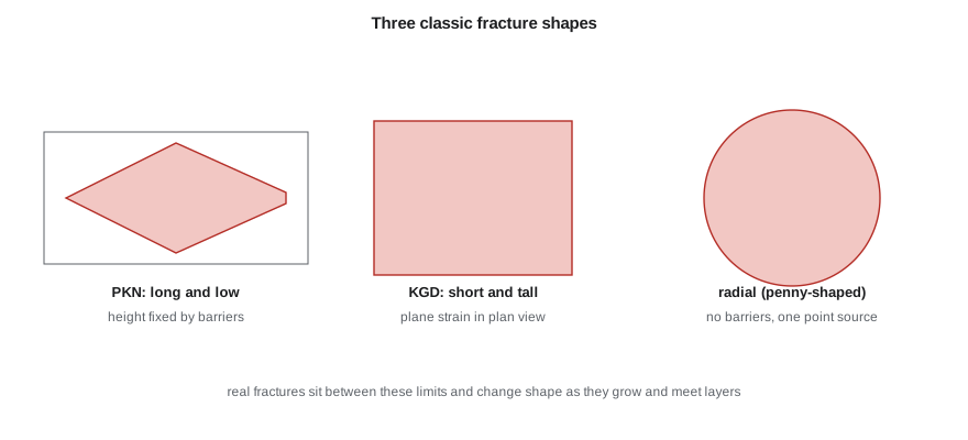
Knowing the stress tells Ethan how a fracture will open. The next question is how big it will get: how long, how tall and how wide, for a given rate, fluid and pumping time. Tom draws three shapes on the whiteboard. 'Every fracture simulator in the industry, from the simplest spreadsheet to the full three-dimensional codes, grew out of these three. Learn them, and you'll know what the software is assuming when it gives you an answer.'

This lesson develops the classic two-dimensional fracture geometry models, PKN and KGD, and the radial model, then adds leak-off, height growth and the effects of many fractures growing at once. It ends with what the models can and cannot tell an engineer about real fractures in horizontal wells.

The ingredients of a geometry model

Any fracture model combines four physical relations. Elasticity links the fracture's width to the net pressure inside it, through the rock's stiffness. Fluid flow along the fracture links the pressure gradient to the flow rate, the width and the fluid's viscosity; for a Newtonian fluid between parallel walls, the pressure drop per unit length is proportional to viscosity times flow rate divided by width cubed. Mass balance says that the volume pumped equals the fracture volume plus the fluid that has leaked into the rock. And a propagation criterion says when the tip advances, involving the rock's toughness. Different models make different simplifying assumptions about shape and about which terms matter.

The PKN model

The Perkins-Kern-Nordgren model, PKN, describes a fracture whose height is fixed, because stress barriers above and below confine it, and whose length is much greater than its height. Each vertical cross-section is treated as an independent crack in plane strain, so it is elliptical, with a maximum width proportional to the local net pressure times the height. Fluid friction along the long fracture controls the pressure, which falls from the wellbore to the tip. In PKN fractures, net pressure rises with time as the fracture grows; a rising net pressure in the field is a sign of a contained, lengthening fracture.

Nordgren's solution for a PKN fracture with no leak-off and a Newtonian fluid gives the half-length and the maximum width at the wellbore as functions of time, where q is the rate into one wing, μ the viscosity, G the shear modulus, ν Poisson's ratio and h the height.

Two features stand out. Length grows almost in proportion to time, while width grows slowly, with the fifth root. And the length is very sensitive to height: halve the height and, for the same volume, the fracture becomes far longer. That is why height containment is the first question in any design.

The KGD model

The Khristianovic-Geertsma-de Klerk model, KGD, assumes the opposite shape: the fracture is tall compared with its length, or is in plane strain in the horizontal plane, so each horizontal cross-section is the same. The width is controlled by the length rather than the height, and the fracture is wider and shorter than a PKN fracture for the same volume. Net pressure in KGD falls with time. KGD suits short fractures in thick zones and is a good model for the early growth of any fracture before it reaches the barriers.

Here qh is the rate per unit height into one wing.

The radial model

When there are no stress barriers and fluid enters at a point, the fracture grows as a circle, or penny. Radial models apply to fractures from a short perforated interval in a thick, uniform zone, and to the early life of many fractures before they reach bounding layers. Once the radius reaches the barriers, a radial fracture changes into a confined PKN-like shape.

Adding leak-off

Real fractures lose fluid through their faces. Carter's leak-off relation, introduced in lesson 7, says the leak-off velocity at each point falls with the square root of the time since that point was opened. Integrating over the fracture faces and over time gives the volume lost. The mass balance then gives a smaller fracture for the same pumped volume. The fluid efficiency, the ratio of fracture volume to pumped volume, falls as leak-off rises. In permeable rock, efficiencies of 20 to 40 percent are common; in very tight rock, efficiencies can be high unless natural fractures take fluid.

Nolte's work in the 1980s gave practical ways to estimate leak-off and efficiency from the pressure decline after a minifrac, and to size the pad, the proppant-free fluid pumped first. A rule from his analysis is that the pad fraction of the job should be roughly (1 − η)/(1 + η), where η is the efficiency, so that the pad has just leaked away when the proppant reaches the tip.

# Fracture geometry: PKN (Nordgren) and KGD (Geertsma-de Klerk) no-leakoff solutions, then a leak-off correction
import math
SI = True   
if SI:   # one cluster on the 03-22 Cardium horizontal
    q_cluster, h, E, nu, mu, t_min = 2.0, 15.0, 20e9, 0.22, 0.004, 40.0     # m3/min, m, Pa, -, Pa.s, min
    CL = 4e-5                                  # Carter leak-off coefficient, m/sqrt(min)
else:    # one cluster on the 3-22H Bakken horizontal (inputs converted to SI inside)
    q_cluster, h, E, nu, mu, t_min = 16.0 * 0.159, 100.0 * 0.3048, 4.0e6 * 6895, 0.25, 0.003, 90.0
    CL = 0.0002 * 0.3048                       # 0.0002 ft/sqrt(min), very tight rock
G = E / (2 * (1 + nu)); t = t_min * 60.0
q = q_cluster / 60.0 / 2                       # one wing, m3/s
def pkn(q, t): return (0.68 * (G * q**3 / ((1 - nu) * mu * h**4)) ** 0.2 * t ** 0.8,
                       2.5 * ((1 - nu) * mu * q**2 / (G * h)) ** 0.2 * t ** 0.2)
def kgd(q, t):
    qh = q / h
    return (0.48 * (8 * G * qh**3 / ((1 - nu) * mu)) ** (1 / 6) * t ** (2 / 3),
            1.32 * (8 * (1 - nu) * mu * qh**3 / G) ** (1 / 6) * t ** (1 / 3))
f = (lambda m: f"{m:,.0f} m") if SI else (lambda m: f"{m/0.3048:,.0f} ft")
fw = (lambda m: f"{m*1000:.1f} mm") if SI else (lambda m: f"{m/0.0254:.2f} in")
for name, fn in (("PKN (height fixed, long fracture)", pkn), ("KGD (short fracture, tall)", kgd)):
    L, w = fn(q, t)
    print(f"{name:34s} half-length {f(L):>9s}, wellbore width {fw(w)}")
# leak-off: reduce the wing until injected volume = fracture volume + leak-off (Carter, fracture growing as t^0.8)
L, w = pkn(q, t)
for _ in range(60):
    V_frac = math.pi / 5 * w * h * L
    leak = 2 * L * h * CL * math.sqrt(t_min) * 1.48 * 2          # two faces; 1.48 accounts for opening time (PKN growth)
    eta = V_frac / (V_frac + leak)
    L = pkn(q * eta, t)[0]; w = pkn(q * eta, t)[1]
print(f"with leak-off: half-length {f(L)}, width {fw(w)}, fluid efficiency about {eta:.0%}")
print("height growth, layered stresses and many clusters sharing fluid make real fractures shorter and more complex than these models")

PKN (height fixed, long fracture)  half-length   1,030 m, wellbore width 4.4 mm
KGD (short fracture, tall)         half-length     476 m, wellbore width 7.1 mm
with leak-off: half-length 759 m, width 3.6 mm, fluid efficiency about 60%
height growth, layered stresses and many clusters sharing fluid make real fractures shorter and more complex than these models

For one cluster on the 04-22, pumping 2 m³/min of slickwater for 40 minutes into a 15 m tall fracture, the PKN model predicts a half-length of about 1,000 m and a width of about 4 mm with no leak-off; KGD, assuming a tall fracture, gives about 480 m. Adding leak-off with a coefficient typical of tight sand cuts the PKN length to about 760 m, with a fluid efficiency of about 60 percent. Tom is unimpressed by the big numbers. 'Microseismic and production data on the 03-22 suggest effective half-lengths of maybe 100 to 150 m. These models assume one fracture with all the cluster's fluid, a perfectly contained height and no complexity. Use them to understand trends, not to predict length.'

Height growth

Height is the least certain dimension and often the most important. A fracture grows in height when its net pressure exceeds the stress contrast with the layers above and below. Stress contrasts of a few megapascals between a sand and a bounding shale usually contain a fracture; smaller contrasts, high net pressures from viscous fluids or high rates, and weak interfaces that the fracture cannot cross all affect the outcome. Pseudo-three-dimensional models calculate height from the layered stress profile at each point along the fracture, and planar three-dimensional models solve the full geometry. Both need a good stress profile from logs calibrated to DFITs.

Height growth matters for three reasons. A fracture that grows out of the pay wastes fluid and proppant and leaves the pay poorly stimulated. A fracture that grows into a water zone can make a well produce mostly water. And regulators and the public want assurance that fractures stay far below fresh groundwater. In practice, measured fracture heights from microseismic monitoring in many basins are tens of metres to a couple of hundred metres, far below shallow aquifers that are usually many hundreds of metres above the target, but the separation must be checked for each well.

Many fractures at once

In a plug-and-perf stage with several clusters, several fractures grow at the same time from the same wellbore. They compete for fluid and they push on each other: each fracture raises the stress around it, a stress shadow that can squeeze its neighbours, especially when clusters are close together. Fractures from the middle clusters may be narrower or curve away, while those at the ends of a stage grow more. Perforation friction, the subject of limited entry in lesson 10, is the main tool for sharing fluid evenly. Fiber-optic measurements and tracers in many basins show that a large fraction of clusters may take little fluid, which is why cluster efficiency is an active research area.

Natural fractures and rock fabric add complexity. In some shales, the hydraulic fracture opens or shears existing natural fractures, creating a network rather than a single planar crack. In others, fractures stay largely planar. The degree of complexity affects how much rock is contacted, how proppant is distributed and how much of the fracture network stays conductive after closure.

What the models are for

Geometry models remain useful when they are used for what they do well. They show how length, width and net pressure respond to rate, viscosity, volume and height; they size pads and proppant schedules; they explain the net pressure record during a job; and, calibrated with measurements, they compare designs on a consistent basis. They are weaker at predicting the absolute length and complexity of fractures in heterogeneous, naturally fractured rock. Modern practice combines models with diagnostics, such as microseismic, fiber optics, tracers, pressure interference between wells and production analysis, to learn what each basin's fractures are really like.

From the models to a design decision

Ethan uses the models for comparisons. Doubling the viscosity in PKN raises the width by about 15 percent and shortens the fracture slightly; doubling the rate per cluster lengthens it by about 50 percent. Lowering the leak-off coefficient raises efficiency and length. Splitting the same stage volume between more clusters shortens each fracture. None of these comparisons needs the absolute length to be right, and all of them help choose between designs. Tom's advice is to pick one model, calibrate it to the measured closure, the treating pressures and any diagnostics from the 03-22, and then use it consistently from well to well.