Equations of state for reservoir fluids

Nadia's compositional model of the deep Tamarack Lake condensate runs on the Peng-Robinson equation of state. 'Every number the simulator produces, from dew points to liquid dropout to separator yields, comes from one cubic equation,' she tells Ethan. 'You should understand it well enough to know when it is lying to you.' She hands him a gas analysis from the Drayton Valley sales meter and asks him to calculate its z-factor with Peng-Robinson and compare it with the DAK result from Lesson 4.

From ideal gas to van der Waals

An equation of state (EOS) relates pressure, volume and temperature for a substance or mixture. The ideal gas law, pV = nRT, is the simplest, and it fails for real fluids because it ignores the size of molecules and the attraction between them. In 1873, van der Waals added two corrections. The constant b, the co-volume, subtracts the volume occupied by the molecules themselves. The constant a reduces the pressure to account for attraction between molecules. The result describes both gas and liquid with one equation, and it predicts a critical point where the two become identical.

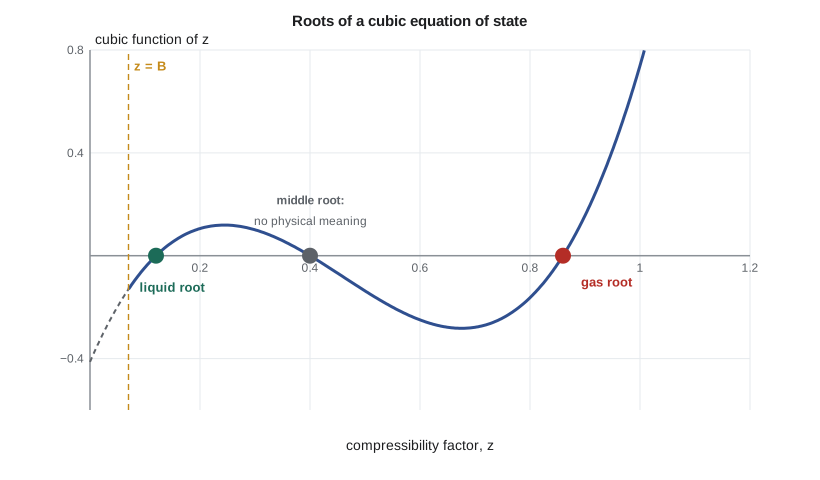
Written in terms of the compressibility factor z = pV/(RT), the van der Waals equation is a cubic polynomial in z. Below the critical temperature, over a range of pressures, the cubic has three real roots. The largest root is the gas z-factor, the smallest is the liquid z-factor, and the middle root has no physical meaning. Above the critical temperature, there is one real root. The constants a and b can be calculated for each pure component from its critical temperature and pressure, by requiring that the critical isotherm has an inflection point with zero slope at the critical point.

CHE-220 Chemical Engineering Thermodynamics I develops cubic equations of state in more depth, with residual properties and fugacity derivations. This lesson focuses on what reservoir engineers need: how the Peng-Robinson equation is applied to petroleum mixtures, and how its predictions are used and checked.

Soave-Redlich-Kwong and Peng-Robinson

The van der Waals equation is qualitatively right but quantitatively poor: it overpredicts liquid volumes and gives poor vapour pressures. Redlich and Kwong (1949) improved the attraction term. Soave (1972) made the attraction parameter a function of temperature through the acentric factor, which gives accurate vapour pressures for hydrocarbons; the resulting Soave-Redlich-Kwong (SRK) equation is still widely used in gas processing. Peng and Robinson (1976) changed the attraction term again to improve liquid density predictions. Their equation, Peng-Robinson (PR), is the most widely used EOS in petroleum engineering and is the default in most compositional reservoir simulators and PVT programs.

For each pure component, the constants come from critical properties and the acentric factor ω. The parameter κ controls how strongly the attraction changes with temperature.

Mixing rules

For a mixture, the EOS constants are combined from the component values using mixing rules. The classical van der Waals rules use a quadratic sum for a and a linear sum for b. Binary interaction parameters, kᵢⱼ, adjust the attraction between unlike molecules. They are zero or small for pairs of hydrocarbons of similar size, larger for methane with heavy components, and important for non-hydrocarbons: carbon dioxide, nitrogen and hydrogen sulphide with hydrocarbons typically have kᵢⱼ of about 0.02 to 0.15. Tuning kᵢⱼ between methane and the heavy fractions is one of the main ways to match a measured saturation pressure.

Solving for z

With dimensionless parameters A = (aα)ₘp/(RT)² and B = bₘp/(RT), the Peng-Robinson equation becomes a cubic in z. It can be solved analytically with Cardano's formula, or numerically with Newton's method starting from z = 1 for the gas root or z = B for the liquid root. When there are three roots, the correct one for a single phase is the one with the lower Gibbs energy; in a two-phase flash, the liquid root is used for the liquid phase and the gas root for the gas phase.

# Peng-Robinson compressibility factor of a natural gas mixture (classical mixing, kij = 0)
import math
SI = True   
R = 10.7316                                   # psia ft3 / (lbmol R)
comp = {  # mole fraction, Tc (R), Pc (psia), acentric factor
    'N2': (0.015, 227.2, 493.1, 0.040), 'CO2': (0.020, 547.6, 1071.0, 0.225),
    'C1': (0.800, 343.0, 667.8, 0.011), 'C2': (0.090, 549.6, 707.8, 0.099),
    'C3': (0.045, 665.7, 616.3, 0.152), 'nC4': (0.030, 765.3, 550.7, 0.200)}

def pr_z(p, T):
    a, b = {}, {}
    for c, (y, tc, pc, w) in comp.items():
        k = 0.37464 + 1.54226 * w - 0.26992 * w**2
        alpha = (1 + k * (1 - math.sqrt(T / tc)))**2
        a[c] = 0.45724 * R**2 * tc**2 / pc * alpha
        b[c] = 0.07780 * R * tc / pc
    am = sum(comp[i][0] * comp[j][0] * math.sqrt(a[i] * a[j]) for i in comp for j in comp)
    bm = sum(comp[i][0] * b[i] for i in comp)
    A, B = am * p / (R * T)**2, bm * p / (R * T)
    c2, c1, c0 = -(1 - B), A - 3 * B**2 - 2 * B, -(A * B - B**2 - B**3)
    z = 1.0
    for _ in range(100):                      # Newton iteration from the gas side
        f = z**3 + c2 * z**2 + c1 * z + c0
        z -= f / (3 * z**2 + 2 * c2 * z + c1)
    return z

T = 180 + 459.67
Mg = sum(y * m for y, m in zip([v[0] for v in comp.values()], [28.01, 44.01, 16.04, 30.07, 44.10, 58.12]))
print(f"gas molar mass {Mg:.2f}, specific gravity {Mg / 28.97:.3f}")
for p in (1000, 2500, 4000):
    z = pr_z(p, T)
    print(f"p {p} psia" + (f" ({p * 6.895 / 1000:.1f} MPa)" if SI else "") + f": Peng-Robinson z = {z:.4f}")

gas molar mass 20.57, specific gravity 0.710
p 1000 psia (6.9 MPa): Peng-Robinson z = 0.8872
p 2500 psia (17.2 MPa): Peng-Robinson z = 0.8277
p 4000 psia (27.6 MPa): Peng-Robinson z = 0.8779

For the sales gas, with molar mass 20.57 kg/kmol and gravity 0.710, Peng-Robinson gives z = 0.887 at 6.9 MPa, 0.828 at 17.2 MPa and 0.878 at 27.6 MPa, at 82 °C. The DAK correlation for a 0.72-gravity gas gave 0.874 at 10.3 MPa and 0.885 at 24.1 MPa, so the two methods agree to within about 1 to 2 percent once the slight difference in gravity is allowed for. Ethan is reassured, and also notes the agreement is good partly because this is a lean gas well away from its critical point.

Volume translation

Peng-Robinson predicts gas densities well, but it typically underpredicts liquid densities of reservoir oils by 5 to 15 percent. Péneloux and co-workers showed that a simple shift of the molar volume, the volume translation, corrects the liquid density without changing the phase equilibrium. Each component has a shift parameter cᵢ, and the corrected molar volume is V − Σ xᵢcᵢ. Because the shift does not affect fugacities, the bubble points and dew points are unchanged. Modern PVT software applies volume translation routinely, and the shift for the heavy pseudo-components is often tuned to match the measured stock-tank oil density or the reservoir oil density from the CCE.

Fugacity and phase equilibrium

The EOS supplies the fugacity coefficient of each component in each phase, which is what the flash calculation of Lesson 10 needs. For Peng-Robinson, the fugacity coefficient has a closed-form expression in terms of z, A, B and the mixture parameters. At equilibrium, the fugacity of each component, its mole fraction times its fugacity coefficient times the pressure, is equal in the gas and liquid. The successive substitution algorithm updates K-values from the ratio of the fugacity coefficients until this condition is met. Bubble point, dew point and full phase envelope calculations follow the same logic.

Calculating a phase envelope

With an EOS and a flash algorithm, the full phase envelope of a reservoir fluid can be calculated. The usual method, due to Michelsen, starts at low pressure on the dew point side, solves for the saturation temperature at successive pressures, and follows the curve around the critical point to the bubble point side, using the slope of the curve to predict each new point. The critical point itself is found where the bubble point and dew point branches meet, or by a direct critical point calculation. Quality lines, for constant liquid fraction, are traced in the same way. Comparing the calculated envelope with the measured saturation pressure at reservoir temperature, and with the separator conditions, is a quick test of whether a fluid model is reasonable before it is used.

Choosing between Peng-Robinson and SRK is mostly a matter of habit and the data available. SRK, used widely in gas processing and in some North Sea studies, predicts vapour pressures and gas properties well, while PR predicts liquid densities somewhat better before volume translation. Once both are characterized and tuned with volume translation, they usually perform similarly. What matters more is that the same EOS, with the same components and parameters, is used consistently in the PVT program, the reservoir simulator and the process simulator, so that a barrel of stock-tank oil in one is the same barrel in the others. Many companies maintain a single tuned fluid model per field for exactly that reason.

A tuned EOS also provides properties that black-oil tables cannot: the enthalpy of each phase for thermal and process calculations, the Joule-Thomson cooling of gas across a choke, the composition of every produced stream, and the behaviour of the reservoir fluid when other gases are injected. Those capabilities are what make compositional simulation worth its higher computing cost for volatile oils, gas condensates and gas injection projects.

Strengths and limits of cubic EOS

Cubic equations of state describe phase equilibrium of hydrocarbon mixtures remarkably well for such simple equations, and they are fast enough to run millions of flashes in a reservoir simulation. Their weaknesses are known. Liquid densities need volume translation. Near the critical point, cubic equations predict the shape of the phase envelope less accurately. They describe water and other polar components poorly without special mixing rules. And above all, their predictions for real reservoir fluids depend on how the heavy fraction is characterized, because the critical properties of the C₇+ pseudo-components are estimated, not measured. More complex equations, such as GERG-2008 for natural gases and the statistical associating fluid theory family, are used for custody transfer and special applications, but cubic EOS remain the workhorse of reservoir engineering.