Vertical curves

A road's profile, like its plan, is a chain of straight grades joined by curves. Where a rising grade meets a falling one, a crest curve rounds off the top so that drivers can see over it; where a falling grade meets a rising one, a sag curve rounds off the bottom so that headlights reach far enough at night and the ride stays comfortable. The engineer picks the length of each curve for sight distance and comfort. The surveyor computes the elevation of every stake along it, finds the high or low point for drainage, and checks that the finished grade matches the design. This lesson covers the parabolic vertical curve that nearly all road and rail designs use.

Why a parabola

A vertical curve is a parabola rather than a circular arc because a parabola's grade changes at a constant rate with horizontal distance. That makes it easy to compute: the elevation at any point is a simple quadratic in the distance from the start of the curve, and the grade at any point is a straight-line function of the same distance. For the flat curves of road design, the difference between a parabola and a circle of similar size is negligible, and the parabola is far more convenient.

The vertical curve is defined on the profile by the point of vertical intersection, PVI, where the two straight grades meet; the incoming grade g1 and outgoing grade g2, in percent; and the curve length L, measured horizontally. The curve is usually symmetric about the PVI, beginning at the BVC (beginning of vertical curve) L/2 before the PVI and ending at the EVC (end of vertical curve) L/2 after it. The algebraic difference of grades is A = |g2 − g1|, and the ratio K = L/A, the horizontal distance needed for a 1 percent change of grade, is the number designers use to set curve lengths for a given design speed.

Here x is the horizontal distance from the BVC. The first two terms are the elevation on the incoming tangent; the third is the offset from that tangent, which grows with the square of x. At the PVI, where x = L/2, the offset is AL/800, which is the external distance E from the PVI down (or up) to the curve. The high or low point, where the grade is zero, exists on the curve only when g1 and g2 have opposite signs.

The coulee crest curve

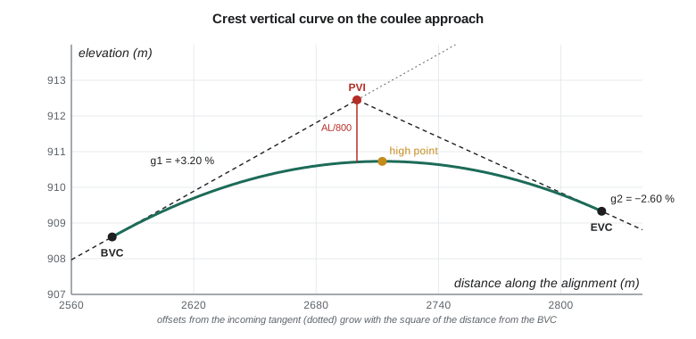
The realigned highway climbs out of the coulee at +3.20 % and then drops toward the canal bridge at −2.60 %. The design puts the PVI at chainage 2+700.000, elevation 912.450, with a curve length of 240 m.

# Crest vertical curve where the realigned highway climbs out of the coulee (metres)
g1, g2 = 3.20, -2.60          # grades in percent
L = 240.0                     # curve length, m
PVI, zPVI = 2700.000, 912.450 # chainage and elevation of the PVI
BVC = PVI - L / 2; EVC = PVI + L / 2
zB = zPVI - g1 / 100 * L / 2
r = (g2 - g1) / 100 / L       # rate of change of grade per metre
fmt = lambda s: f"{int(s // 1000)}+{s % 1000:07.3f}"
def z(x):                     # elevation at chainage x on the curve
    t = x - BVC
    return zB + g1 / 100 * t + r * t * t / 2
A = abs(g2 - g1); K = L / A
print(f"BVC {fmt(BVC)} {zB:.3f}   EVC {fmt(EVC)} {z(EVC):.3f}   A {A:.2f} %   K {K:.1f}")
t_hi = -g1 / 100 / r          # where the grade is zero
print(f"high point at {fmt(BVC + t_hi)}  elevation {z(BVC + t_hi):.3f}")
print(" chainage      tangent    offset     curve")
x = BVC
while x <= EVC + 1e-6:
    tang = zB + g1 / 100 * (x - BVC)
    print(f"{fmt(x)}  {tang:9.3f}  {z(x)-tang:8.3f}  {z(x):9.3f}")
    x += 40
# Check grade at the bridge abutment stake, 30 m past the PVI
xb = PVI + 30
print(f"grade at {fmt(xb)}: {100*(g1/100 + r*(xb-BVC)):.2f} %  elevation {z(xb):.3f}")

BVC 2+580.000 908.610   EVC 2+820.000 909.330   A 5.80 %   K 41.4
high point at 2+712.414  elevation 910.729
 chainage      tangent    offset     curve
2+580.000    908.610     0.000    908.610
2+620.000    909.890    -0.193    909.697
2+660.000    911.170    -0.773    910.397
2+700.000    912.450    -1.740    910.710
2+740.000    913.730    -3.093    910.637
2+780.000    915.010    -4.833    910.177
2+820.000    916.290    -6.960    909.330
grade at 2+730.000: -0.43 %  elevation 910.691

The BVC is at 2+580.000, elevation 908.610, and the EVC at 2+820.000, elevation 909.330. The algebraic difference is 5.80 %, so K is 41.4: the curve uses 41.4 m of road for each percent of grade change. The high point is at 2+712.414, elevation 910.729, a little past the PVI because the incoming grade is steeper than the outgoing one. At the PVI the curve is 910.710, exactly 1.740 m below the PVI, which is AL/800. The table lists tangent elevations along the incoming grade extended, the offsets from it, and the curve elevations; each offset is four times the offset at half the distance, as the square law requires.

The high point matters for drainage. Water on the road surface runs away from it in both directions, so the ditches and any curb inlets must be arranged on each side, and the surveyor marks it on the stakes. On a crest curve with a very small grade change, the road near the high point is almost flat over a long distance, and the designers must make sure that cross slope alone will drain the surface.

The last line checks the bridge approach: 30 m past the PVI, at 2+730, the grade is already −0.43 % and the elevation 910.691. The bridge's design profile must start from exactly this elevation and grade, and Theo compares the highway profile with the bridge drawings at the abutment before any stakes go in.

Unequal tangents and other cases

Most vertical curves are symmetric, but where the profile is tightly constrained, for example between a bridge deck and an intersection, the designer may use an asymmetric curve with different lengths on each side of the PVI. It is computed as two parabolas that share a common tangent at a point above the PVI, and design software handles it routinely. The surveyor's checks are the same: the elevations at the BVC and EVC must match the tangents, the grade must be continuous through the join, and the high or low point must be where the drainage plan expects it.

Two vertical curves sometimes overlap a horizontal curve, and on a well-designed highway they usually do, with the vertical curve lying within the horizontal one. That does not complicate the profile computation, which is always done along the stationing, but it does mean the stake for a given station gives both an offset position from the horizontal alignment and an elevation from the vertical one. Superelevation, the banking of the road on a curve, adds a third component: the edges of the road are higher or lower than the centreline by the cross slope times the half-width, and the cross slope changes through the transition from normal crown to full superelevation.

Sight distance and the length of curve

The surveyor does not choose curve lengths, but knowing why they are what they are helps in checking a design and in explaining a change in the field. On a crest curve, the limiting factor is sight distance: a driver's eye must be able to see an object on the road far enough ahead to stop. With the driver's eye height and the object height fixed by the design guide, the minimum curve length for a given stopping sight distance depends only on A, which is why design guides tabulate minimum K values by design speed. On a sag curve in daylight there is no sight problem, so the limit is headlight reach at night, and on sag curves under bridges, the clearance to the structure. A crest curve that is too short for its design speed is a real hazard, not a matter of style.

This also explains a common field conversation. When a contractor asks whether a curve can be shortened to save a cut, the answer depends on whether the shorter curve still meets the K value for the design speed; the surveyor can compute the new elevations in minutes, but the decision belongs to the designer. Ruth's crews never change a profile on their own authority, however small the change, and they record every design change they receive with its date and its source.

For the coulee curve, a minimum K of 40 for the design speed would require at least 232 m of curve; the design's 240 m is just above it. That is typical: a designer usually picks the shortest curve that meets the standard and fits the terrain, with a little margin, and rounds to a convenient length.

Grade stakes and cut and fill

The grading crew does not need a table of elevations; it needs marks on the ground that say how far to cut or fill. The surveyor's grade stakes, or the machine-control model in Lesson 6, give that information. A traditional grade stake is set at an offset from the edge of the work, so it survives the earthmoving, and is marked with the station, the offset, and the cut or fill from the top of the stake (or from a mark on a lath beside it) to the design grade at the corresponding point on the road. The cut or fill is the ground or stake elevation minus the design elevation: positive is cut, negative is fill.

For example, at 2+700 the curve elevation on the centreline is 910.710. A grade stake at 15 m right, where the design subgrade is 0.36 m lower because of the cross slope and pavement thickness, is at 911.420 on top. The design subgrade there is 910.350, so the stake reads C 1.070: cut 1.07 m below the top of the stake. A crew reading stakes must know whether the numbers refer to finished grade, subgrade or some other surface, and the stake must say so.

Checking the profile in the field

Once the road is graded, the surveyor checks it against the profile. Levels or GNSS shots on the subgrade at each station and offset are compared with the design elevations, and the differences reported. A systematic difference along the whole curve usually means a wrong benchmark or a mistake in the vertical datum; a difference that grows with distance from the BVC usually means a wrong grade or curve length was used; a scatter of small differences is normal grading tolerance. Lessons 11 and 12 return to the statistics of these checks.

Vertical control is the foundation of all of this. The profile is only as good as the benchmarks the stakes are set from, and Ruth insists on a closed level loop through the work area before the first grade stake, and on re-checking the benchmarks after any heavy equipment has worked near them.

Profiles for pipes and canals

The same ideas apply to gravity pipes and canals, which are usually straight grades between changes, without curves. For the siphon in Lesson 8 and the pump station's discharge pipe, the critical numbers are the invert elevations at each change of grade and the grade itself, often a fraction of a percent. A 0.20 % grade falls only 2 mm per metre, so a small error in a benchmark or a rod reading is a large fraction of the fall between two joints. Pipe crews use lasers set to the design grade inside the pipe, and the surveyor's job is to set the laser's starting point and grade, check it daily, and check the inverts as the pipe goes in.