Structural monitoring with GNSS and sensors

Periodic surveys show where a structure was on the days the crew measured it. Continuous monitoring shows how it behaves between those days: how the dam crest rises and falls with the seasons, how fast it settles in the years after the rebuild, and whether anything sudden happens. Continuous GNSS receivers, tiltmeters, crack meters, piezometers and other sensors, logged automatically and sent to the office, make this possible. This lesson covers how the data are collected, how a time series is modelled to separate trend, seasonal cycles and noise, and how alert levels are applied so that a real change is noticed without false alarms every week.

Continuous GNSS on structures

A continuous GNSS monitoring station is a geodetic receiver and antenna on a stable mount on the structure, logging data all the time and sending it to a server. The data are processed against one or more reference stations off the structure, on stable ground, using the relative methods of GEOM-300, to give the monitoring antenna's position relative to the reference. Short baselines, a few hundred metres to a few kilometres, keep the atmospheric errors nearly identical at both ends so that they cancel.

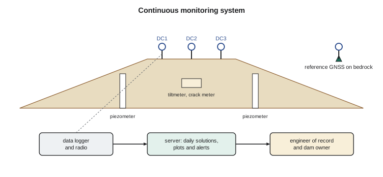
Processing choices set the precision. Positions computed every second from RTK give a few centimetres; daily static solutions from 24 hours of data give a millimetre or two horizontally and two or three millimetres vertically, because averaging over a day removes much of the short-period noise from multipath and atmosphere. For a dam that settles a few millimetres a year, daily solutions are the right product; for a bridge deck that moves under traffic and wind, the high-rate solutions are what matter.

Antenna mounts must not add their own movement. A steel mast heats and bends in the sun, a concrete pillar can tilt, and anything attached to a structure moves with it in ways that may not represent the structure as a whole. The district's crest stations sit on short reinforced-concrete pillars cast into the crest, with forced-centring mounts, and their antennas are never removed without a recorded procedure, because a change of antenna or a slight shift in its height creates a step in the series that can be mistaken for movement.

Sensors that complement GNSS

GNSS gives three-dimensional position at a few points. Other sensors fill in what it cannot see. Tiltmeters, small electrolytic or accelerometer-based sensors bolted to a wall or pier, measure rotation to a few microradians, which shows the gate piers leaning slightly as the reservoir fills. Crack meters and joint meters measure the opening of a crack or joint to a hundredth of a millimetre. Piezometers measure water pressure inside the embankment and its foundation, which the engineers use to check seepage and stability. Inclinometers, read by hand or with in-place sensors, measure lateral movement at depth. Weather stations record air temperature, solar radiation and rainfall, which explain much of the movement the other sensors see.

Each sensor has its own units, calibration and failure modes. A vibrating-wire piezometer reads a frequency that is converted to pressure with a calibration supplied by the manufacturer, corrected for temperature and barometric pressure; a tiltmeter reads a voltage converted to an angle, with a zero that may drift. The surveyor who manages the system must know these conversions and check them, because a sensor error looks exactly like a structural change on a plot.

Tilt and displacement are linked by the height over which the tilt acts: a tilt of 150 microradians over a 12 m pier gives about 1.8 mm of movement at the top. Comparing the top movement from the prisms in Lesson 9 with the tilt measured by the tiltmeter is a useful cross-check between two quite different instruments.

Modelling a time series

Two years of daily heights from crest station DC2 form a time series with three ingredients: a long-term trend (the crest settling slowly as the rebuilt embankment consolidates), a seasonal cycle (the crest rising and falling with temperature, reservoir level and frost), and noise (the scatter of the daily solutions). Fitting a model with all three by least squares separates them and gives each a number with an uncertainty.

Here v is the velocity, the rate of settlement; A is the amplitude of the annual cycle; and e is the residual, what is left when trend and cycle are removed. The residuals should look like random noise. If they show a pattern, such as a step, a curve or a second cycle, the model is missing something real, and the engineers need to know about it.

import math, random
# Dam crest GNSS station DC2: two years of daily heights (mm), trend + annual cycle + noise, fitted by least squares
random.seed(42)
days = list(range(0, 730))
true_v, true_amp = -3.0, 4.0                          # mm per year settlement, mm annual amplitude
h = [true_v * t / 365.25 + true_amp * math.cos(2 * math.pi * (t - 200) / 365.25) + random.gauss(0, 2.5) for t in days]
# Model: h = a + v t + c cos(wt) + s sin(wt); normal equations solved by Gaussian elimination
w = 2 * math.pi / 365.25
rows = [[1.0, t / 365.25, math.cos(w * t), math.sin(w * t)] for t in days]
N = [[sum(r[i] * r[j] for r in rows) for j in range(4)] for i in range(4)]
b = [sum(r[i] * y for r, y in zip(rows, h)) for i in range(4)]
M = [N[i] + [b[i]] for i in range(4)]
for c in range(4):
    p = max(range(c, 4), key=lambda r: abs(M[r][c])); M[c], M[p] = M[p], M[c]
    for r in range(4):
        if r != c:
            f = M[r][c] / M[c][c]; M[r] = [x - f * y for x, y in zip(M[r], M[c])]
a, v, cc, ss = [M[i][4] / M[i][i] for i in range(4)]
res = [y - (a + v * r[1] + cc * r[2] + ss * r[3]) for r, y in zip(rows, h)]
rms = math.sqrt(sum(e * e for e in res) / (len(res) - 4))
print(f"velocity {v:+.2f} mm/yr, annual amplitude {math.hypot(cc, ss):.2f} mm, residual RMS {rms:.2f} mm")
# Alert check on the last 7 days against fixed thresholds from the monitoring plan (relative to the baseline fit)
last7 = sum(res[-7:]) / 7
for name, lim in (('alert', 8.0), ('alarm', 15.0)):
    print(f"7-day mean residual {last7:+.1f} mm vs {name} level {lim:.0f} mm: {'exceeded' if abs(last7) > lim else 'ok'}")
# A sudden 12 mm drop on day 730 would be caught at once by a single-day test?
print(f"single-day 3-sigma limit {3*rms:.1f} mm; a 12 mm step {'is' if 12 > 3*rms else 'is not'} flagged on the first day")

velocity -3.30 mm/yr, annual amplitude 4.12 mm, residual RMS 2.48 mm
7-day mean residual +1.3 mm vs alert level 8 mm: ok
7-day mean residual +1.3 mm vs alarm level 15 mm: ok
single-day 3-sigma limit 7.4 mm; a 12 mm step is flagged on the first day

The fit gives a velocity of −3.30 mm per year, the crest settling, and an annual amplitude of 4.12 mm, with a residual RMS of 2.48 mm. The simulated data were built with a true velocity of −3.0 mm per year and an amplitude of 4.0 mm, so the estimates are close but not exact, which is a reminder that two years is a short series for separating a trend from a cycle of similar size. With more years, the velocity estimate tightens considerably.

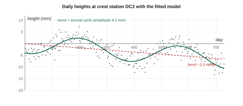
Without the annual term, a fit of the trend alone would give a different velocity, because whatever part of a cycle the series happens to start and end in pulls the straight line up or down. A series that starts in a summer high and ends in a winter low would show settlement even if there were none. This is the single most common mistake in reading monitoring plots, and it is why the model always includes the seasonal term for any series longer than a few months.

Alerts without false alarms

A monitoring system is only useful if someone acts on what it shows, and people stop acting on alarms that ring every week. So alert rules are designed to catch real changes quickly while rarely triggering on noise. Two common approaches are thresholds on smoothed values and statistical limits on individual values. A 7-day mean of the residuals compared with fixed alert and alarm levels, here 8 and 15 mm, reacts to sustained changes while ignoring single bad days. A limit of three times the residual RMS on single days catches sudden large events at once.

In the code, the last week's mean residual is +1.3 mm, far below the 8 mm alert level, so nothing is triggered. The single-day limit is 7.4 mm, three times the RMS, so a sudden 12 mm drop, such as a slump in the crest, would be flagged on the first day, while a 5 mm drop would have to persist for several days before the weekly mean caught it. Every rule is a compromise between speed and false alarms, and the monitoring plan says which the engineers prefer for each point.

Alerts also need a human response chain. The monitoring plan states who receives an alert, how quickly they must respond, what checks they make first (is it a sensor fault, a processing problem, a known event such as a reservoir drawdown?), and when the engineer of record and the dam owner must be told. Ruth's team tests the chain twice a year with a simulated alert, because the first real one is a bad time to discover that a phone number has changed.

Data management

A continuous system produces a lot of data: dozens of sensors, readings every few minutes, and GNSS files every day, for decades. The data must be stored with full metadata (sensor, location, calibration, units, changes of equipment), processed in a documented and repeatable way, backed up, and kept available for the life of the structure. A reading without its calibration record is worthless twenty years later, when the engineers want to compare the dam's behaviour with its first filling. The district's system stores raw data, processed values and every change to the processing, so that any number in a report can be traced back.

Power and communications fail, especially in winter on a remote site. The system must log locally when the radio link is down and send the backlog when it returns, and the server must alarm when a sensor stops reporting, not just when a value is high. Silence from a sensor is itself information: it may mean a dead battery, or it may mean the instrument has been damaged by the very movement it was supposed to measure.

Monitoring of dams in Alberta follows the province's dam and canal safety rules and the Canadian Dam Association's guidelines, which expect owners to have surveillance programs proportional to the dam's consequence classification. The district's engineer sets the program's scope; the surveyor delivers measurements of known quality on time.

Combining measurements

The real value of a monitoring system comes from looking at the measurements together. If the crest GNSS stations show the crest rising in spring while the piezometers show pressures rising as the reservoir fills, and the tiltmeters show the gate piers leaning slightly downstream, all three are telling the same story, and the engineers can compare it with the behaviour the design predicted. If one instrument disagrees with the rest, it is either a fault in that instrument or something local happening at its location, and either one needs a visit. The district's dashboard shows the reservoir level, the air temperature and the main sensors on one time axis for exactly this reason.