Quality control

Every lesson in this course has ended with checks: the deflection to the PT, the diagonals of a building, the check shots on a subgrade, the test of a movement. This lesson pulls those habits together into a quality system for an engineering survey: the planned set of procedures, checks and records that make sure the survey's products are right and that anyone can see why they are right. Quality control is not a final inspection added at the end; it is built into every step, from the instruments in the truck to the files delivered to the owner. The lesson finishes with the project's final quality review of the bridge approach stakeout.

Quality assurance and quality control

Two terms are used together and are worth keeping apart. Quality assurance is the system: the procedures, training, equipment management and records that are designed to produce good work. Quality control is the checking: the measurements and reviews that test whether a particular product meets its specification. A firm with good quality assurance still needs quality control on every job, because systems fail; and quality control without a system catches errors one at a time, after they have been made.

On large public projects, the roles are often split. The contractor's surveyor does the layout and its quality control; the owner's surveyor, or an independent firm, does quality assurance checks, re-measuring a sample of the contractor's work. For the headworks project, Coulee Geomatics is the owner's surveyor: it did the design survey and the control, and it checks the contractor's layout and does the as-builts. Ruth's quality plan for the job describes both its own procedures and the checks it makes on others.

Instruments

Quality starts with instruments that do what they claim. Total stations, levels and GNSS receivers drift out of adjustment and get knocked about in trucks. Each instrument has a calibration record: periodic calibration by a qualified service, and field checks by the crew at set intervals. For total stations, the field checks include the collimation and trunnion axis errors (measured by observing in both faces), the vertical index error, the optical or laser plummet, and the electronic distance measurement on a calibration baseline. Levels get a two-peg test. GNSS receivers and their antennas are checked by occupying a known control point and comparing.

The ISO 17123 series of standards gives field procedures for testing surveying instruments, part by part: levels, theodolites, distance meters, total stations and GNSS RTK. In Canada, calibration baselines for distance meters are maintained in several regions, and provincial survey associations publish guidance on their use. Ruth's crews follow the ISO procedures, simplified where appropriate, and file the results in each instrument's record.

Accessories matter as much as instruments. A tribrach with a loose clamp, a prism with the wrong constant entered, a bent pole, a bubble out of adjustment: each causes errors that no amount of care with the instrument will cure. The crew checks pole bubbles weekly, keeps prism constants in a list taped inside the instrument case, and replaces tribrachs that fail the plummet check.

Procedures and redundancy

The second part of quality is procedure. Every measurement that matters should be made in a way that reveals its own errors: angles in both faces, distances both ways, levels in closed loops, GNSS points occupied twice at different times, traverses closed on known points, layout points checked from a second setup. This redundancy is the surveyor's main tool, and least squares (GEOM-220) is the way to use it: an adjustment with redundant observations gives not only the best answer but its precision and a test of whether any observation is a blunder.

Written procedures make redundancy routine. The project's survey procedures manual sets out, for each kind of work, the instruments, the observing method, the checks, the tolerances and the records. New crew members learn from it; experienced ones follow it on the hard days when shortcuts are tempting. When something goes wrong, the procedure is reviewed as well as the work.

Statistics of checks

Checks produce numbers, and the numbers need interpretation. Three statistics come up again and again. The mean of a set of check differences shows bias: a systematic offset, such as a wrong benchmark, a wrong antenna height, or a wrong prism constant. The standard deviation shows precision: how much the checks scatter about their mean. And the root mean square error combines both, measuring how far the checks are from zero on average. A set of checks with a small standard deviation and a large mean is precise but biased, and the cause must be found.

Accuracy is often reported at 95 % confidence. For a single dimension, such as height, the 95 % accuracy is 1.96 times the RMSE if the errors are normal and unbiased. For horizontal position, combining east and north errors, the US National Standard for Spatial Data Accuracy uses a factor of 1.7308 times the horizontal RMSE, which is also widely used elsewhere. GEOM-310 and GEOM-350 used the newer ASPRS standards for mapping products; for stakeout and as-builts, the contract's tolerances and these simpler statistics are usually enough.

Acceptance by percent within limits

Highway agencies often accept work by percent within limits, PWL. A random sample of measurements is taken from a lot of work, the mean and standard deviation are computed, and the normal distribution is used to estimate what fraction of the whole lot lies within the specification limits. If the PWL is above a set level, often 90 %, the lot is accepted at full pay; below it, the pay may be reduced or the work rejected. The same idea works for survey quality: it asks what proportion of the staked points is likely to be within tolerance, not just whether the sample points are.

Here U and L are the upper and lower limits and Φ is the standard normal cumulative distribution. Agencies' own PWL methods often use a quality index and tables based on the sample size rather than the normal approximation; the idea is the same.

The bridge approach check

Before the contractor's paving crew starts on the bridge approach, Coulee Geomatics re-measures a random sample of 25 of the contractor's staked points, independently, from different control. The differences, re-measured minus staked, are the data for the quality check.

import math
# Quality control: independent check of 25 staked points on the bridge approach (re-measured minus staked, mm)
dE = [3, -2, 5, 1, -4, 2, 6, -1, 0, 3, -3, 4, 2, -5, 1, 7, -2, 0, 3, 2, -1, 4, 1, -3, 2]
dN = [-1, 2, -3, 4, 1, -2, 0, 3, -4, 1, 2, -1, 5, 0, -2, 1, 3, -1, 2, -3, 1, 0, -2, 4, 1]
dH = [4, -6, 2, 8, -3, 5, 1, -2, 7, 3, -4, 6, 0, 2, -5, 9, 1, -1, 4, 3, -2, 5, 2, -3, 6]
n = len(dE)
mean = lambda v: sum(v) / len(v)
sd = lambda v: math.sqrt(sum((x - mean(v)) ** 2 for x in v) / (len(v) - 1))
rmse = lambda v: math.sqrt(sum(x * x for x in v) / len(v))
rh = math.sqrt(rmse(dE) ** 2 + rmse(dN) ** 2)
print(f"E: mean {mean(dE):+.1f} sd {sd(dE):.1f} RMSE {rmse(dE):.1f} | N: mean {mean(dN):+.1f} sd {sd(dN):.1f} RMSE {rmse(dN):.1f} mm")
print(f"horizontal RMSE {rh:.1f} mm -> 95 % horizontal accuracy (NSSDA factor 1.7308) {1.7308*rh:.1f} mm")
print(f"vertical: mean {mean(dH):+.1f} sd {sd(dH):.1f} RMSE {rmse(dH):.1f} mm -> 95 % vertical (1.96) {1.96*rmse(dH):.1f} mm")
t = mean(dH) / (sd(dH) / math.sqrt(n))
print(f"vertical bias t = {t:.2f} vs 2.06 (24 df): {'bias present - check the benchmark or rod' if abs(t) > 2.06 else 'no bias'}")
# Percent within limits (PWL) for a +/-10 mm vertical tolerance, using the normal model
phi = lambda z: 0.5 * (1 + math.erf(z / math.sqrt(2)))
m, s = mean(dH), sd(dH)
pwl = 100 * (phi((10 - m) / s) - phi((-10 - m) / s))
print(f"PWL for +/-10 mm: {pwl:.1f} % (acceptance needs 90 %): {'accept' if pwl >= 90 else 'reject or re-stake'}")
radial = [math.hypot(a, b) for a, b in zip(dE, dN)]
print(f"points over 8 mm radial: {sum(r > 8 for r in radial)} of {n}")

E: mean +1.0 sd 3.1 RMSE 3.2 | N: mean +0.4 sd 2.4 RMSE 2.4 mm
horizontal RMSE 4.0 mm -> 95 % horizontal accuracy (NSSDA factor 1.7308) 6.9 mm
vertical: mean +1.7 sd 4.2 RMSE 4.4 mm -> 95 % vertical (1.96) 8.6 mm
vertical bias t = 2.02 vs 2.06 (24 df): no bias
PWL for +/-10 mm: 97.5 % (acceptance needs 90 %): accept
points over 8 mm radial: 0 of 25

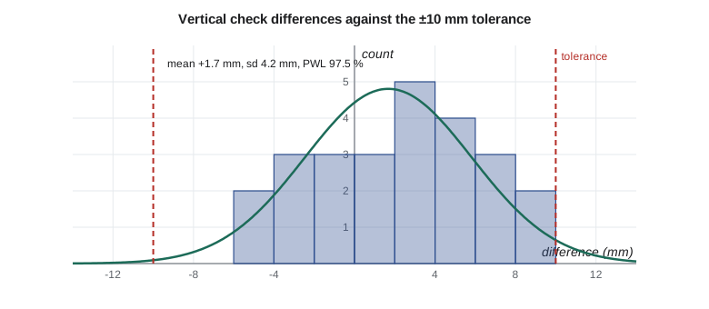
Horizontally, the checks have means of +1.0 mm east and +0.4 mm north, standard deviations of 3.1 and 2.4 mm, and a horizontal RMSE of 4.0 mm, which gives a 95 % horizontal accuracy of 6.9 mm. None of the 25 points is more than 8 mm from its check position. Vertically, the mean is +1.7 mm, the standard deviation 4.2 mm and the RMSE 4.4 mm, giving a 95 % vertical accuracy of 8.6 mm. The t-statistic for the vertical mean is 2.02, just below the 95 % critical value of 2.06 for 24 degrees of freedom: there is no statistically significant bias, but it is close, and Ruth notes it for the next check. The PWL for a ±10 mm vertical tolerance is 97.5 %, above the 90 % acceptance level, so the stakeout is accepted.

The analysis also says what it cannot. Twenty-five points cannot detect a problem that affects only a few stakes, such as a single disturbed hub, so the quality plan also requires the contractor's own checks on every stake and spot checks of anything that looks wrong. Statistics tells whether a process is working; it does not replace looking.

Records and traceability

A quality system lives in its records. For every product, it should be possible to trace back to the field data, the instruments and their calibration, the control used, the procedures followed, the checks made and the people who made and reviewed it. That traceability is what lets Ruth answer a question three years from now about why a stake was where it was, and it is what an auditor or a court will ask for if something goes wrong. The firm's file for each job holds the raw data, the processed data, the check results, the field notes and photographs, and the sign-offs.

Professional obligations reinforce this. Alberta Land Surveyors and professional engineers working in the province are expected to have quality management practices proportionate to their work, and the professional associations publish practice standards that include record keeping. Many firms also follow ISO 9001 for quality management, and some public owners require it of their consultants.

Learning from errors

Errors will happen, even with a good system. The difference between a firm that improves and one that does not is what happens next. Ruth's practice is a short, blame-free review of any error that reaches a client or the field: what happened, why the checks did not catch it, and what change to procedure, training or equipment would catch it next time. The antenna-height error of Lesson 6 led to a new rule that every machine's antenna height is measured and recorded by the surveyor, not taken from a sticker. The skewed bearing spacing of Lesson 7, which nearly went to the field as a square dimension on a superintendent's sketch, led to a standard note on every bridge layout sheet.

At the end of the headworks project, Ruth's team holds a project review: what went well, what went badly, and what to keep for the next job. The control report, the procedures, the quality plan and the lessons learned all go into the firm's templates. The siphon broke through 11 mm left of its target, inside the budget of Lesson 8. The bridge girders fitted. The pump bases were fixed before the pumps arrived. And the district now has as-built records it can trust for the life of the structures.