Data processing

By the end of the berth survey, the launch has logged about 400 million soundings, along with positions, attitudes, sound speed casts, water levels and the operator's notes. None of it is yet a product. Processing turns raw measurements into a surface the client can design with and a chart compiler can trust: it applies every correction, removes the soundings that are not the seabed, combines the rest into a gridded surface with an uncertainty for every cell, and documents what was done. Leah has processed lidar for two years; hydrographic processing follows the same logic but has its own tools, its own errors and its own standards of proof.

The processing chain

The chain begins with conversion: the raw files from the sonar, the navigation system and the sound speed probe are read into processing software, and each data stream is checked for gaps, spikes and time jumps. Next come the corrections: the post-processed navigation solution (Lesson 6) replaces the real-time one; the vessel configuration, with its lever arms and calibration biases (Lesson 7), is applied; each ping is ray-traced through the nearest sound speed profile (Lesson 3); and depths are reduced to the vertical datum, either through water levels and zoning or through GNSS heights and the separation model (Lessons 2 and 6). The result is a georeferenced point cloud with a total propagated uncertainty attached to every sounding. Only then does cleaning begin.

Because the corrections are applied in software from the raw data, any of them can be changed and the data reprocessed: a better sound speed cast, a revised separation model, a corrected lever arm. Leah keeps the raw files untouched and records every setting, so that the final surface can be traced back, step by step, to the measurements. That traceability is what the charting office will audit.

Total propagated uncertainty

Each sounding's uncertainty is computed by propagating the uncertainties of every input through the equations that produce its position and depth. The inputs include the GNSS position and height, the heading, roll and pitch, the lever arms and their measurement accuracy, the timing, the sound speed at the transducer and through the water column, the sonar's range and angle measurement, and, in a tide-reduced survey, the water level and its zoning. Models published in the literature, and implemented in commercial software, combine these into a vertical and a horizontal uncertainty for each sounding at a stated confidence. The result shows the expected pattern: soundings near nadir are the most certain, those at the outer edge of the swath much less so, and soundings collected far from a sound speed cast or in rough weather less so again.

Gridding with uncertainty

Hundreds of millions of soundings are reduced to a gridded surface, typically with cells 0.5 to 2 m on a side for a harbour survey, smaller where objects must be resolved. A simple grid would average the soundings in each cell, but averaging mixes good and bad soundings, smooths away real shoals and ignores the uncertainty that has been so carefully computed. Modern hydrographic software uses uncertainty-aware algorithms. The most widely used, CUBE (Combined Uncertainty and Bathymetry Estimator), developed at the University of New Hampshire's Center for Coastal and Ocean Mapping, estimates depth at each grid node from nearby soundings weighted by their uncertainty and their distance. Where soundings disagree, because some come from the seabed and others from a fish school or a multipath echo, it keeps several hypotheses about the depth and chooses among them, reporting the chosen depth, its uncertainty and the alternatives.

import math, random
random.seed(360)
# Soundings in four 2 m cells of the berth: (cell, depth m, 1-sigma TPU m); one cell has a fish school and a spike
data = []
true = {'A': 15.52, 'B': 15.61, 'C': 15.74, 'D': 15.40}
for cell, z in true.items():
    for k in range(40):
        u = random.choice((0.05, 0.07, 0.10))          # nadir beams better than outer beams
        data.append((cell, random.gauss(z, u), u))
data += [('C', 12.9 + 0.1 * k, 0.07) for k in range(6)]   # fish school 3 m above the bottom
data += [('D', 17.85, 0.10)]                                 # a multipath spike below the bottom

def cube_like(sound, gate=3.0):
    """Sequential hypothesis tracking in the spirit of CUBE: each sounding joins the nearest
    hypothesis within gate*sigma or starts a new one; hypotheses keep weighted means."""
    hyps = []
    for z, u in sound:
        best = None
        for h in hyps:
            s = math.sqrt(1.0 / h['w'] + u * u)
            if abs(z - h['z']) <= gate * s and (best is None or abs(z - h['z']) < abs(z - best['z'])):
                best = h
        if best is None:
            hyps.append({'z': z, 'w': 1.0 / u ** 2, 'n': 1})
        else:
            w = 1.0 / u ** 2
            best['z'] = (best['z'] * best['w'] + z * w) / (best['w'] + w); best['w'] += w; best['n'] += 1
    return sorted(hyps, key=lambda h: -h['n'])

def tvu(d, a, b): return math.sqrt(a * a + (b * d) ** 2)
for cell in 'ABCD':
    s = [(z, u) for c, z, u in data if c == cell]
    hy = cube_like(s)
    h = hy[0]
    # Reported uncertainty: the larger of the propagated error of the mean and the scatter about it
    near = [z for z, u in s if abs(z - h['z']) < 0.5]
    sd = math.sqrt(sum((z - h['z']) ** 2 for z in near) / (len(near) - 1))
    unc = max(1.0 / math.sqrt(h['w']), sd) * 1.96
    others = ', '.join(f"{x['z']:.2f} m (n={x['n']})" for x in hy[1:]) or 'none'
    print(f"cell {cell}: {len(s)} soundings, chosen {h['z']:.2f} m (n={h['n']}), 95 % {unc:.2f} m; "
          f"other hypotheses: {others}")
    print(f"        allowed TVU: Special Order {tvu(h['z'], 0.25, 0.0075):.2f} m, Exclusive {tvu(h['z'], 0.15, 0.0075):.2f} m")
# A median filter would also catch the spike, but would it keep a real 1 m boulder? That is the hydrographer's call.

cell A: 40 soundings, chosen 15.53 m (n=40), 95 % 0.13 m; other hypotheses: none
        allowed TVU: Special Order 0.28 m, Exclusive 0.19 m
cell B: 40 soundings, chosen 15.62 m (n=40), 95 % 0.12 m; other hypotheses: none
        allowed TVU: Special Order 0.28 m, Exclusive 0.19 m
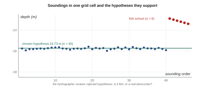
cell C: 46 soundings, chosen 15.73 m (n=40), 95 % 0.18 m; other hypotheses: 13.05 m (n=4), 13.35 m (n=2)
        allowed TVU: Special Order 0.28 m, Exclusive 0.19 m
cell D: 41 soundings, chosen 15.38 m (n=40), 95 % 0.14 m; other hypotheses: 17.85 m (n=1)
        allowed TVU: Special Order 0.28 m, Exclusive 0.19 m

In cells A, B and D the soundings agree, and the estimator returns one hypothesis each, with 95 percent uncertainties of 0.12 to 0.14 m. In cell C a fish school passed under the launch: six soundings 2.3 to 2.8 m above the bottom form two small hypotheses, while 40 soundings support the seabed at 15.73 m. In cell D, a single multipath echo at 17.85 m forms its own hypothesis and is outvoted. All four cells meet the Special Order allowance of 0.28 m at this depth; cell C's 0.18 m only just meets the Exclusive Order's 0.19 m, because the fish school's soundings were mixed into the cell's scatter. Real CUBE is more elaborate, propagating each sounding's influence to nearby nodes, tracking hypotheses with a filter and using several disambiguation rules, but the idea is the same.

Cleaning: what to reject

Not every sounding is the seabed. Fish, kelp, bubbles under the hull, propeller wash from passing ships, side-lobe returns, multipath echoes off a wharf face, and electrical or acoustic interference all produce soundings that must be rejected. Automatic filters do most of the work: they reject soundings outside depth limits, beyond a chosen beam angle, with poor quality flags from the sonar, or far from a local surface. Gridding algorithms like CUBE then isolate most of the remaining noise. But the hydrographer must review the result, area by area, in plan view, profile and three dimensions, looking especially at the places where the algorithm had to choose: where hypotheses compete, where the surface has spikes, and where the uncertainty is high.

The rule that governs cleaning is shoal-biased caution: a sounding shallower than its neighbours is not rejected merely because it is inconvenient. A single shoal sounding in an area where the multibeam swath crossed an old wharf may be a pile stub or a block of concrete. The hydrographer looks at it from several lines, checks the backscatter and the side-scan record, and, if it might be real, flags it for development: the launch goes back and surveys it at slow speed with the object near nadir. Rejecting a real obstruction is far worse than keeping a fish.

Quality control

Several checks tell whether the survey is internally consistent and meets its specification. Cross lines, run across the main lines, are compared with the gridded surface built from the main lines; the differences, analysed by beam angle, reveal sound speed and calibration errors and measure the repeatability of the system. Overlapping lines are compared with each other; areas where they disagree point to problems with a particular line or a particular time. The grid's uncertainty layer is compared, cell by cell, with the allowance for the specified order, and the coverage layer shows any holes. Junctions with previous surveys and with other platforms, such as the lidar on the reservoir margins, are compared in their overlap. Automated tools now perform many of these checks and produce statistics and maps for the report.

For the berth, Leah runs the cross-line comparison and finds a mean difference of 0.01 m and a 95 percent spread of 0.09 m, well within the allowance. The overlap analysis shows one afternoon with a slight smile in the outer beams, which she traces to a river plume that arrived between casts; reprocessing those lines with the next cast removes it. The coverage map shows three small holes near the wharf face, where the launch could not get close; they are filled by a pole-mounted multibeam line run at high water.

Features and the final surface

Besides the depth surface, a charting survey delivers features: wrecks, obstructions, rocks, piles, pipelines and anything else a mariner should know about, each with its position, least depth, how it was found and how sure the surveyor is. Features are attributed according to the charting office's feature specification and delivered in its format. The surface itself is delivered as a grid with depth and uncertainty layers, often at more than one resolution, together with the cleaned soundings, the side-scan mosaic, the backscatter mosaic and a descriptive report that explains the survey, its methods, its problems and its results.

The CHS reviews submitted surveys against its standards and guidelines before using them on charts. The review checks the metadata, the datums, the uncertainty and coverage statistics, and the treatment of features; a survey that cannot show how its depths were derived is unlikely to be used for charting, however good it looks.

Merging sources

On the reservoir, the final surface merges three sources: last autumn's topobathymetric lidar for the margins, this autumn's single-beam lines for the deep pool, and the land survey above the water line. Each comes with its own uncertainty and density. Leah aligns them to the same vertical datum, checks them against each other in their overlaps, and combines them with a weighted method that favours the more certain source where they overlap and blends smoothly across the boundary. In the 3 to 6 m band the lidar and the sonar agree to a mean of 0.04 m, the sonar slightly deeper, consistent with the sonar's high frequency reflecting from the top of the soft sediment while the lidar's green light returns from about the same surface. The merged surface feeds the capacity table in Lesson 11.