Feature extraction

Engineers do not design from point clouds. They design from surfaces, lines and objects: the plane of a pier face, the axis and diameter of a pipe, the edge of a canal lining, the centreline of a road, the attachment points of a power line. Feature extraction turns millions of points into a few dozen parameters that describe such shapes, with known accuracy. At the headworks Ines needs pier faces and their lean, the gate house pipework, the deck edges and the gate arms; along the canal she needs breaklines at the top and toe of each bank, culvert inverts, fence lines and poles. This lesson covers the main tools: fitting geometric primitives, robust estimation with RANSAC, region growing and segmentation, and extracting lines and edges.

Fitting a plane by least squares

A plane can be written \(\mathbf{n}\cdot\mathbf{p} + d = 0\) with unit normal \(\mathbf{n}\). The best-fitting plane through a set of points, minimizing the sum of squared perpendicular distances, passes through their centroid, and its normal is the eigenvector of the smallest eigenvalue of the points' covariance matrix: exactly the computation used for the planarity feature of lesson 7. The smallest eigenvalue divided by the number of points gives the mean squared distance from the plane, a measure of flatness and noise. This orthogonal fit treats all three coordinates alike, which is right for scan data where errors are roughly isotropic, unlike the ordinary regression that minimizes vertical distances only.

Least squares assumes that every point belongs to the plane and that errors are small and random. Real scans of a pier face include the handrail, a person standing on the deck, debris lodged against the pier, and points on the adjacent gate. Even a few such outliers pull a least-squares plane away from the true surface. The surface must first be separated from everything else.

RANSAC: random sample consensus

RANSAC, published by Fischler and Bolles in 1981, is a robust method that finds a model supported by the largest group of points while ignoring the rest. It repeats a simple trial: choose the minimum number of points needed to define the model at random (three for a plane), compute the model, and count the points that lie within a tolerance of it, the inliers. After many trials the model with the most inliers wins, and it is refined by least squares on its inliers alone. The number of trials needed for confidence \(p\) of drawing at least one sample free of outliers, when a fraction \(w\) of points are inliers and each sample has \(s\) points, is

For a plane with 77 percent inliers, eight trials give 99 percent confidence; with only 30 percent inliers, 169 are needed; and models with more parameters need far more. The tolerance must suit the data's noise: too tight and real surface points are rejected, too loose and nearby clutter joins the plane.

import math, random
random.seed(8)
Z0 = 900.0
def plane3(p, q, r):
    u = [q[i] - p[i] for i in range(3)]; v = [r[i] - p[i] for i in range(3)]
    n = [u[1]*v[2] - u[2]*v[1], u[2]*v[0] - u[0]*v[2], u[0]*v[1] - u[1]*v[0]]
    m = math.sqrt(sum(x * x for x in n))
    if m < 1e-9: return None
    n = [x / m for x in n]; return n, -sum(n[i] * p[i] for i in range(3))

# Upstream face of the headworks pier: 3.0 m wide, 4.0 m tall, leaning 0.4 deg, plus clutter
lean = math.radians(0.4)
pts = [[random.uniform(0, 3), 0.6 + z * math.tan(lean) + random.gauss(0, 0.002), Z0 + z]
       for z in [random.uniform(0, 4) for _ in range(400)]]
pts += [[random.uniform(0, 3), random.uniform(0.2, 1.5), Z0 + random.uniform(0, 4)] for _ in range(120)]  # handrail, debris, people

# RANSAC: how many trials for 99 % confidence with 400 / 520 inliers and 3-point samples
w = 400 / 520; need = math.ceil(math.log(1 - 0.99) / math.log(1 - w ** 3))
print(f"inlier fraction {w:.2f}: {need} trials give 99 % confidence")
best = (0, None)
for _ in range(max(need, 50)):
    m = plane3(*random.sample(pts, 3))
    if not m: continue
    n, d = m
    inl = [p for p in pts if abs(sum(n[i] * p[i] for i in range(3)) + d) < 0.006]
    if len(inl) > best[0]: best = (len(inl), m, inl)
cnt, (n, d), inl = best
# refine with least squares on the inliers: y = a + b z (the face is nearly x-z)
zs = [p[2] - Z0 for p in inl]; ys = [p[1] for p in inl]
zm, ym = sum(zs) / len(zs), sum(ys) / len(ys)
b = sum((z - zm) * (y - ym) for z, y in zip(zs, ys)) / sum((z - zm) ** 2 for z in zs); a = ym - b * zm
rms = math.sqrt(sum((y - (a + b * z)) ** 2 for z, y in zip(zs, ys)) / len(zs))
print(f"RANSAC inliers {cnt}; refined lean {math.degrees(math.atan(b)):.3f} deg (true 0.400), out of plumb {b*4000:.1f} mm over 4 m, RMS {rms*1000:.1f} mm")

# Pipe in the gate house: circle fit (Kasa) to a slice of points around a 0.457 m diameter pipe
cx, cy, r0 = 2.150, 1.320, 0.2285
sl = [(cx + r0 * math.cos(t) + random.gauss(0, 0.002), cy + r0 * math.sin(t) + random.gauss(0, 0.002))
      for t in [random.uniform(math.radians(100), math.radians(260)) for _ in range(60)]]   # only the near side is visible
Sx = sum(x for x, y in sl); Sy = sum(y for x, y in sl); n_ = len(sl)
Sxx = sum(x*x for x, y in sl); Syy = sum(y*y for x, y in sl); Sxy = sum(x*y for x, y in sl)
Sxz = sum(x*(x*x+y*y) for x, y in sl); Syz = sum(y*(x*x+y*y) for x, y in sl); Sz = sum(x*x+y*y for x, y in sl)
# normal equations for x^2 + y^2 + D x + E y + F = 0
Mx = [[Sxx, Sxy, Sx], [Sxy, Syy, Sy], [Sx, Sy, n_]]; rhs = [-Sxz, -Syz, -Sz]
def solve3(M, b):
    M = [r[:] + [v] for r, v in zip(M, b)]
    for c in range(3):
        piv = max(range(c, 3), key=lambda r: abs(M[r][c])); M[c], M[piv] = M[piv], M[c]
        for r in range(3):
            if r != c:
                f = M[r][c] / M[c][c]; M[r] = [x - f * y for x, y in zip(M[r], M[c])]
    return [M[i][3] / M[i][i] for i in range(3)]
D, E, F = solve3(Mx, rhs)
xc, yc = -D / 2, -E / 2; rr = math.sqrt(xc * xc + yc * yc - F)
print(f"pipe axis at ({xc:.4f}, {yc:.4f}), diameter {2*rr*1000:.1f} mm (true 457.0) from a {160} deg arc")

inlier fraction 0.77: 8 trials give 99 % confidence
RANSAC inliers 396; refined lean 0.393 deg (true 0.400), out of plumb 27.5 mm over 4 m, RMS 2.0 mm
pipe axis at (2.1489, 1.3201), diameter 454.3 mm (true 457.0) from a 160 deg arc

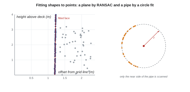
The pier face in the code leans 0.4° and is surrounded by 120 clutter points among 520. Eight trials would give 99 percent confidence; the code runs 50 for safety, finds 396 inliers, and the refined fit gives a lean of 0.393°, which is 27.5 mm out of plumb over the 4 m face, with a residual RMS of 2.0 mm matching the scanner's noise. This is the measurement the engineers wanted: is the second pier leaning? Lesson 9 compares the two piers. The circle fit recovers a 457 mm pipe's axis to within a millimetre or two and its diameter as 454.3 mm from a 160° arc, the near side only, because the wall hides the back of the pipe. Partial arcs weaken a circle fit, especially its radius, so the fit should be checked against the pipe's nominal size and, where possible, by scanning from a second side.

Other primitives: cylinders, spheres and lines

Industrial and structural scenes are full of simple shapes. A sphere has four parameters (centre and radius) and is fitted for registration targets (lesson 5). A circle in a known plane has three; a cylinder in space has five (axis direction, a point on the axis, and radius). A practical method for pipes, used in the code, slices the cloud perpendicular to the approximate axis, fits circles to each slice, and fits a line through the circle centres to find the axis; a rigorous fit then adjusts all five parameters together by nonlinear least squares. Cones, tori (for pipe elbows) and planes complete most piping and steelwork libraries. Each fit reports its residuals and the standard deviations of its parameters, which tell the modeller whether the shape really is a cylinder: a residual pattern that varies around the circumference suggests an oval or dented pipe, worth knowing for a 70-year-old penstock.

Lines in three dimensions, such as the edges of the deck or the top of a wall, are found by intersecting fitted planes, which is more accurate than picking points on the edge itself, because mixed pixels blur every edge. A deck edge computed as the intersection of the deck top plane and the deck face plane is located to a millimetre or two even though no scan point lies exactly on it.

Segmentation and region growing

RANSAC finds one model at a time. A scene with hundreds of surfaces needs segmentation: dividing the cloud into groups of points that belong to the same surface or object. Region growing starts from a seed point with low curvature, adds neighbours whose normals differ by less than an angle threshold and whose distance from the growing surface is small, and continues until no more points qualify; then a new seed starts the next region. Region growing finds smooth surfaces of any shape, curved or flat, and separates them at sharp edges. Other approaches include clustering by Euclidean distance, which separates objects that do not touch, such as poles from the ground once the ground is removed; supervoxel methods that group points into small homogeneous units first; and the deep learning instance segmentation methods that label each object individually.

Segmentation produces candidates that a modeller then turns into objects. Along the canal, Theo segments the non-ground points into clusters, then tests each cluster: a vertical cylinder about 0.3 m in diameter and 8 to 12 m tall is a pole; a narrow vertical plane 1 to 2 m tall following a line is a fence or sign; a thin horizontal plane spanning the canal is a bridge deck. Rules like these, combined with imagery, populate the district's asset inventory with 340 poles, 61 culverts, 18 turnouts and 9 check structures.

Breaklines and edges from airborne and mobile data

For terrain the most valuable features are breaklines: the lines where slope changes sharply, such as the top and toe of a canal bank, the edge of a road and the shoreline of the reservoir. Breaklines can be digitized manually from the point cloud, using profiles and shaded views, or extracted semi-automatically by finding where the slope or curvature of the bare-earth surface changes sharply and tracing the change along the feature. Water-edge breaklines are often digitized from intensity or imagery, because water returns are sparse. Each breakline vertex needs a correct elevation, taken from nearby ground points rather than from the noisy points at the edge.

Mobile mapping data add road features: lane markings, found by their high intensity on the road surface; curbs and pavement edges, found as small height steps; signs, found as small vertical planes with high retroreflective intensity; and road surface condition, measured as rutting and roughness along profiles. Specialized software extracts many of these automatically, and transportation agencies use them to maintain inventories and pavement management systems.

Accuracy of extracted features

A fitted feature is often more accurate than any single point, because it averages many. The standard deviation of a plane's offset is roughly the point noise divided by the square root of the number of points, so a pier face fitted to 400 points with 2 mm noise is located to about 0.1 mm in a purely statistical sense. In practice the accuracy is limited by registration and control (lesson 5), systematic scanner errors and how well the surface matches the model: a pier face that is not truly flat has no single correct plane. Ines reports extracted dimensions with the registration accuracy, not the statistical fit, and states the model's assumptions, such as 'face modelled as a plane; departures up to 6 mm from that plane shown in the deviation map'.