Registration

Each of the 46 setups at the headworks produced a point cloud in its own scanner frame, with its origin at the scanner and its axes wherever the instrument happened to point. Before anything can be measured across setups, the scans must be brought into one common frame: the process called registration. When the common frame is the project coordinate system, tied to control, the process is often called georeferencing. Registration is the step where a scanning project is most easily ruined without anyone noticing, so Leah reviews it with as much care as Theo spends performing it.

The rigid-body transformation

Two scans of a rigid structure differ by a rotation and a translation. A point \(\mathbf{p}\) in scan 2's frame becomes

in the common frame, where \(\mathbf{R}\) is a 3 × 3 rotation matrix with three independent angles and \(\mathbf{t}\) a translation vector: six parameters in all. Unlike the seven-parameter similarity transformation of GEOM-340 there is no scale factor, because a calibrated scanner measures true distances; a significant scale difference between scans is a sign of a problem, not a parameter to estimate. If the scans are levelled with the instrument's compensator, the rotation reduces to a single angle about the vertical axis, and four parameters suffice, which strengthens the solution.

Registration is the problem of finding \(\mathbf{R}\) and \(\mathbf{t}\) for every scan. There are two broad approaches: matching identified targets or features whose correspondence is known, and matching the surfaces themselves without known correspondences.

Target-based registration

Targets are objects whose centre can be located precisely in a scan: spheres, whose centre is found by fitting a sphere to the points on them; flat checkerboard or black-and-white targets, whose centre is found from the intensity pattern; and, for long ranges, retroreflective targets. A sphere looks the same from every direction, which makes it ideal for joining setups on different sides of a target; a flat target is more precise when seen face-on but degrades at oblique angles. Each target is identified in every scan that sees it, and the scans are linked through common targets.

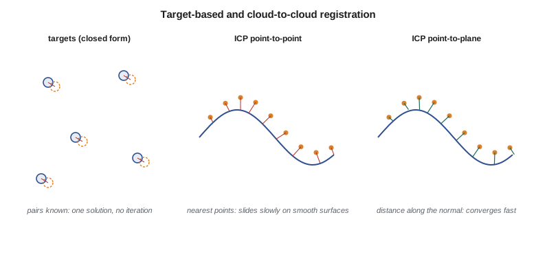
With three or more pairs of corresponding points, the best rotation and translation in the least-squares sense can be computed in closed form, without iteration or approximate values. Several equivalent methods exist; one widely used solution, published by Horn in 1987, represents the rotation as a unit quaternion and finds it as the eigenvector of a 4 × 4 matrix built from the centred coordinates. The translation then follows from the centroids:

Residuals at the targets, the distances between transformed and reference positions, are the first quality measure. Leah expects residuals of a few millimetres for sphere targets within 30 m; a residual several times larger than the rest usually means a target was disturbed, misidentified or partly occluded.

With many scans the problem becomes a network, like a traverse network in surveying. Each pair of overlapping scans gives a link, and a global least-squares adjustment, sometimes called a bundle or network adjustment of the scans, finds all the transformations at once, distributing errors and giving statistics for each link. Control targets measured by total station are included as fixed or weighted points, which ties the whole network to the project coordinates and prevents errors accumulating along a long chain of setups, just as tying a traverse to control at both ends prevents error growing along it.

Cloud-to-cloud registration and ICP

Targets cost time to place and must be visible from several setups. Where scans overlap generously on surfaces with varied geometry, the surfaces themselves can be matched. The classic method is the iterative closest point algorithm (ICP), described by Besl and McKay and by Chen and Medioni in the early 1990s. Starting from an approximate alignment, ICP repeats three steps: for each point in the moving scan find the nearest point in the reference scan; compute the rigid transformation that best aligns these pairs; apply it. The pairs are only guesses, but each iteration improves them, and if the start is close enough the process converges.

Two versions are common. In point-to-point ICP the error is the distance between paired points, and the transformation is computed in closed form as for targets. In point-to-plane ICP the error is the distance from each moving point to the tangent plane at its partner, measured along the surface normal. Point-to-plane allows points to slide along a surface without penalty, which is right, because two scans never sample exactly the same spots, and it converges much faster on smooth surfaces. Its solution needs a linearization for small rotations and is solved by least squares, like the adjustments of GEOM-220.

import math, random
def T(A): return [list(r) for r in zip(*A)]
def mul(A, B): return [[sum(a * b for a, b in zip(r, c)) for c in zip(*B)] for r in A]
def inv(A):
    n = len(A); M = [list(map(float, r)) + [1.0 if i == j else 0.0 for j in range(n)] for i, r in enumerate(A)]
    for c in range(n):
        p = max(range(c, n), key=lambda r: abs(M[r][c])); M[c], M[p] = M[p], M[c]
        d = M[c][c]; M[c] = [x / d for x in M[c]]
        for r in range(n):
            if r != c:
                f = M[r][c]; M[r] = [x - f * y for x, y in zip(M[r], M[c])]
    return [r[n:] for r in M]
def diag(v): return [[v[i] if i == j else 0.0 for j in range(len(v))] for i in range(len(v))]
def col(v): return [[x] for x in v]
def sub(a, b): return [x - y for x, y in zip(a, b)]
def mean(P): return [sum(p[i] for p in P) / len(P) for i in range(3)]
def qmat(q):
    w, x, y, z = q
    return [[w*w+x*x-y*y-z*z, 2*(x*y-w*z), 2*(x*z+w*y)],
            [2*(x*y+w*z), w*w-x*x+y*y-z*z, 2*(y*z-w*x)],
            [2*(x*z-w*y), 2*(y*z+w*x), w*w-x*x-y*y+z*z]]
def mv(M, v): return [sum(M[i][j]*v[j] for j in range(3)) for i in range(3)]

def jacobi_max(A, sweeps=30):
    """Eigenvector of the largest eigenvalue of a symmetric matrix (cyclic Jacobi)."""
    n = len(A); A = [r[:] for r in A]; V = [[float(i == j) for j in range(n)] for i in range(n)]
    for _ in range(sweeps):
        for p in range(n - 1):
            for q in range(p + 1, n):
                if abs(A[p][q]) < 1e-15: continue
                th = 0.5 * math.atan2(2 * A[p][q], A[q][q] - A[p][p]); c, s = math.cos(th), math.sin(th)
                for k in range(n):
                    akp, akq = A[k][p], A[k][q]; A[k][p], A[k][q] = c*akp - s*akq, s*akp + c*akq
                for k in range(n):
                    apk, aqk = A[p][k], A[q][k]; A[p][k], A[q][k] = c*apk - s*aqk, s*apk + c*aqk
                for k in range(n):
                    vkp, vkq = V[k][p], V[k][q]; V[k][p], V[k][q] = c*vkp - s*vkq, s*vkp + c*vkq
    i = max(range(n), key=lambda i: A[i][i])
    return [V[k][i] for k in range(n)]

def horn(A, B):
    """Closed-form rigid transformation B ~ R A + t (Horn 1987, unit quaternion)."""
    ca, cb = mean(A), mean(B)
    S = [[0.0]*3 for _ in range(3)]
    for a, b in zip(A, B):
        a, b = sub(a, ca), sub(b, cb)
        for i in range(3):
            for j in range(3): S[i][j] += a[i] * b[j]
    (Sxx, Sxy, Sxz), (Syx, Syy, Syz), (Szx, Szy, Szz) = S
    N = [[Sxx+Syy+Szz, Syz-Szy, Szx-Sxz, Sxy-Syx],
         [Syz-Szy, Sxx-Syy-Szz, Sxy+Syx, Szx+Sxz],
         [Szx-Sxz, Sxy+Syx, -Sxx+Syy-Szz, Syz+Szy],
         [Sxy-Syx, Szx+Sxz, Syz+Szy, -Sxx-Syy+Szz]]
    q = jacobi_max(N)
    R = qmat(q)
    t = sub(cb, mv(R, ca))
    return R, t

# Five sphere targets seen from scan 2 (scanner coordinates) and their project coordinates
random.seed(5)
true_k = math.radians(37.2); c, s = math.cos(true_k), math.sin(true_k)
Rt = [[c, -s, 0], [s, c, 0], [0, 0, 1]]; tt = [10612.330, 20288.415, 900.0 + 3.112]
A = [[12.1, 3.4, -1.2], [-8.6, 9.9, 0.4], [-15.2, -6.3, 2.8], [4.4, -14.7, -0.9], [20.3, -2.2, 5.1]]
B = [[x + random.gauss(0, 0.002) for x in sub(mv(Rt, a), [-v for v in tt])] for a in A]
R, t = horn(A, B)
print("rotation about z {:.4f} deg; translation {:.3f} {:.3f} {:.3f}".format(math.degrees(math.atan2(R[1][0], R[0][0])), *t))
res = [math.dist([x + y for x, y in zip(mv(R, a), t)], b) * 1000 for a, b in zip(A, B)]
print("target residuals (mm):", " ".join(f"{r:.1f}" for r in res), f" RMS {math.sqrt(sum(r*r for r in res)/len(res)):.1f}")

# ICP on a small cloud (a patch of the coulee bank): scan 3 starts from a rough placement
f = lambda x, y: 0.5 * math.sin(x) + 0.4 * math.cos(1.3 * y)
P = [[x * 0.05, y * 0.05, f(x * 0.05, y * 0.05)] for x in range(-64, 65) for y in range(-64, 65)]  # dense reference scan
h = 0.05; normal = {}
for p in P:                          # normal from the analytic slope of the patch, as a fitted surface would give
    gx = (f(p[0] + h, p[1]) - f(p[0] - h, p[1])) / (2 * h); gy = (f(p[0], p[1] + h) - f(p[0], p[1] - h)) / (2 * h)
    m = math.sqrt(gx * gx + gy * gy + 1); normal[tuple(p)] = [-gx / m, -gy / m, 1 / m]
cell = 0.2; grid = {}
for p in P: grid.setdefault((math.floor(p[0] / cell), math.floor(p[1] / cell)), []).append(p)
def nearest(q):
    i, j = math.floor(q[0] / cell), math.floor(q[1] / cell)
    cand = [p for a in (-1, 0, 1) for b in (-1, 0, 1) for p in grid.get((i + a, j + b), [])]
    return min(cand or P, key=lambda p: math.dist(p, q))
k = math.radians(2.0); c, s = math.cos(k), math.sin(k)
S3 = [[x * 0.4 + 0.13, y * 0.4 + 0.07] for x in range(-6, 7) for y in range(-6, 7)]        # scan 3 samples other spots
Q = [[c*u - s*w + 0.12, s*u + c*w - 0.08, f(u, w) + 0.05 + random.gauss(0, 0.003)] for u, w in S3]
def run_icp(plane, iters=30):
    cur = [q[:] for q in Q]
    for it in range(1, iters + 1):
        pairs = [nearest(q) for q in cur]
        if not plane:
            R, t = horn(cur, pairs)
            cur = [[x + y for x, y in zip(mv(R, q), t)] for q in cur]
        else:
            # point-to-plane: linearized for small rotations w and translation t
            Nm = [[0.0] * 6 for _ in range(6)]; u = [0.0] * 6
            for q, p in zip(cur, pairs):
                n = normal[tuple(p)]
                a = [q[1]*n[2] - q[2]*n[1], q[2]*n[0] - q[0]*n[2], q[0]*n[1] - q[1]*n[0]] + n
                r = sum((qi - pi) * ni for qi, pi, ni in zip(q, p, n))
                for i in range(6):
                    u[i] -= a[i] * r
                    for j in range(6): Nm[i][j] += a[i] * a[j]
            x = [row[0] for row in mul(inv(Nm), col(u))]
            wx, wy, wz, tx, ty, tz = x
            cur = [[q[0] - wz*q[1] + wy*q[2] + tx, wz*q[0] + q[1] - wx*q[2] + ty, -wy*q[0] + wx*q[1] + q[2] + tz] for q in cur]
    return cur
truth = [[u, w, f(u, w)] for u, w in S3]
err = lambda C: math.sqrt(sum(math.dist(a, b)**2 for a, b in zip(C, truth)) / len(C)) * 1000
print(f"true error of scan 3 before ICP: {err(Q):.0f} mm")
for iters in (5, 10, 30):
    print(f"after {iters:2d} iterations: point-to-point {err(run_icp(False, iters)):6.1f} mm, point-to-plane {err(run_icp(True, iters)):5.1f} mm")

rotation about z 37.2034 deg; translation 10612.329 20288.414 903.111
target residuals (mm): 3.8 4.3 3.6 1.6 1.5  RMS 3.2
true error of scan 3 before ICP: 166 mm
after  5 iterations: point-to-point  109.7 mm, point-to-plane   4.2 mm
after 10 iterations: point-to-point   79.9 mm, point-to-plane   4.2 mm
after 30 iterations: point-to-point   65.5 mm, point-to-plane   4.2 mm

With five sphere targets the closed-form solution recovers the rotation of 37.2° and the translation to the millimetre, with target residuals of 1.5 to 4.3 mm and an RMS of 3.2 mm, consistent with the 2 mm noise added to each target. The ICP example registers a patch of the coulee bank whose second scan starts 166 mm out of place. After 30 iterations point-to-point ICP has stalled with the patch still 65 mm wrong, because pairing each point with the nearest sampled point drags the surfaces together slowly and stops in a false minimum. Point-to-plane ICP reaches 4 mm in five iterations, essentially the noise level. The grid index used to find nearest points, which divides the plane into 0.2 m cells and searches only nearby cells, is a small version of the spatial indexes (k-d trees and octrees) that make real registration software fast.

When ICP fails

ICP needs a good starting position, usually within a fraction of the overlap's size and a few degrees of rotation. Software gets one from targets, from the scanner's own sensors (compass, GNSS, inclinometer and inertial sensors in some instruments), from user-picked matching points or from automatic feature matching. ICP also needs geometry that constrains all six parameters. A flat floor constrains height and two tilts but lets the scans slide freely in plan; a long straight tunnel or a canal reach constrains everything except movement along its axis. Such degenerate geometry produces registrations that converge with tiny residuals yet are wrong along the unconstrained direction. The defence is to check registrations against independent information: targets not used in the registration, control, or features in other directions.

Vegetation, moving objects and change also disturb ICP. Leaves move between scans, vehicles and people appear in one scan and not another, and on the coulee bank the surface itself may have changed between epochs, which is exactly what the monitoring wants to detect. Robust versions of ICP reject pairs whose distance exceeds a threshold, and for monitoring the registration is computed only on stable areas, such as bedrock or structures known not to move, so that real change is not absorbed into the transformation.

Georeferencing to control

Registering scans to each other gives a consistent model in an arbitrary frame; georeferencing places it in project coordinates. At the headworks the control targets surveyed by Grant's crew are included in the network adjustment with their coordinates and standard deviations, so that the final transformation of every scan honours the control. Leah checks two things: the residuals at control targets, which should match the combined accuracy of the survey and the scans, and the residuals at checkpoints, targets surveyed but withheld from the adjustment. On this project the control residuals average 2.8 mm and the four checkpoints differ by 3 to 6 mm, comfortably within the 10 mm the engineers need.

For mobile and airborne data the equivalent of registration is the trajectory and strip adjustment of lessons 3 and 4, and the equivalent of georeferencing is the use of ground control. Combining data sets, such as placing the terrestrial scans of the headworks into the airborne point cloud, requires that both be in the same coordinate reference system, realization, epoch and height datum, followed by a check on common surfaces; a residual difference of a few centimetres between them is normal and should be reported.

Reporting registration quality

A registration report gives the method, the number of scans and links, the targets used and their residuals, the overlap and RMS of each cloud-to-cloud link, the control and checkpoint residuals, and any scans excluded or re-registered. Registration software often reports a single number such as mean target error or cloud-to-cloud RMS, which is easily misread. A small cloud-to-cloud RMS shows that the overlapping surfaces fit each other, not that the result is correct in coordinates. Only checks against independent control show absolute accuracy.