Mobile mapping systems

In GEOM-300 the crew drove a rented mobile mapping vehicle along the canal access road to collect lidar for the new canal design. The district now wants the same kind of survey of the whole 24 km main canal: the road, the canal prism, the check structures, culverts and turnouts, the fences, the power line that follows the canal for 6 km, and every sign and gate. A terrestrial scanner would need hundreds of setups; an aircraft would see the canal but not the undersides of bridges or the faces of structures. Ines books a mobile mapping system for two days and plans the survey with Theo.

What a mobile mapping system is

A mobile mapping system mounts one or more laser scanners, several cameras and a navigation system on a moving platform: a vehicle, a rail car, a boat, an all-terrain vehicle or a backpack. The scanners usually measure in a single plane, sweeping a profile across the road at high rate, and the platform's motion spreads successive profiles along the route. Because the platform moves, its position and orientation must be known at every instant, typically 200 times a second or more. A GNSS receiver supplies position; an inertial measurement unit (IMU), with three accelerometers and three gyroscopes, supplies orientation and bridges gaps in GNSS; and a wheel odometer, the distance measuring instrument, helps the inertial solution when the satellites are blocked. The combined navigation solution is called the trajectory.

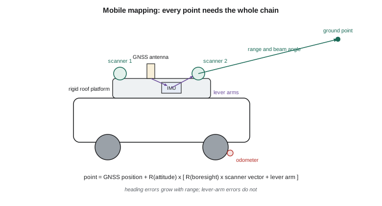
Systems range from survey-grade vehicles costing as much as a house, with two long-range scanners and a navigation-grade IMU, to backpack and handheld systems that use simultaneous localization and mapping (SLAM) instead of GNSS. SLAM estimates the platform's path by matching each new scan to the map built so far; it works indoors and under dense canopy where GNSS fails, but its errors grow with distance travelled unless the path closes loops or passes control. For the canal Ines chooses a vehicle system with two scanners mounted at angles so that one profile sweeps forward and down across the road and the other backward, which reduces shadows behind poles and signs.

The georeferencing equation

Each point measured by a mobile scanner is computed from a chain of measurements and calibrated offsets. In vector form,

where \(\mathbf{r}_{GNSS}(t)\) is the position of the GNSS antenna at the instant \(t\) of the laser measurement, \(\mathbf{R}_b^m(t)\) the rotation from the vehicle body frame to the mapping frame given by roll, pitch and heading from the IMU, \(\mathbf{R}_s^b\) the boresight rotation between the scanner's axes and the IMU's axes, \(\mathbf{r}_s\) the point in the scanner frame from range and beam angle, and \(\mathbf{a}\) the lever arm from the antenna to the scanner's origin, measured in the body frame. In practice the trajectory is referenced to the IMU and there are separate lever arms from IMU to antenna and from IMU to each scanner, but the structure is the same. The airborne equation in lesson 4 is identical.

Every term carries error into the point. Position errors from GNSS pass straight through. Attitude errors are multiplied by range: a heading error of 0.05° moves a point 18 m away by about 16 mm sideways, and a point 50 m away by 44 mm. Lever-arm errors are not multiplied by range but are transferred directly, rotated by the attitude. Boresight errors behave like attitude errors and must be calibrated (lesson 10). Timing matters too: the vehicle travels 2.2 cm in a millisecond at 80 km/h, so all sensors are synchronized to GNSS time to microseconds.

import math
def rot(roll, pitch, yaw):
    """Body-to-mapping rotation, angles in degrees (z-y-x order)."""
    r, p, y = (math.radians(a) for a in (roll, pitch, yaw))
    cr, sr, cp, sp, cy, sy = math.cos(r), math.sin(r), math.cos(p), math.sin(p), math.cos(y), math.sin(y)
    return [[cy*cp, cy*sp*sr - sy*cr, cy*sp*cr + sy*sr],
            [sy*cp, sy*sp*sr + cy*cr, sy*sp*cr - cy*sr],
            [-sp,   cp*sr,            cp*cr]]
def mv(M, v): return [sum(M[i][j]*v[j] for j in range(3)) for i in range(3)]
def add(a, b): return [x + y for x, y in zip(a, b)]

# Vehicle state from the GNSS/INS at one instant (project grid, heights above the vertical datum)
gnss = [10520.412, 20310.885, 900.0 + 12.940]   # antenna position
att = (1.10, -0.80, 63.50)                       # roll, pitch, heading, degrees
lever = [-0.312, 0.055, -0.884]                  # antenna to scanner origin, body frame, m
bore = (0.012, -0.020, 0.035)                    # scanner-to-body boresight angles, degrees
# One return: range 18.400 m, beam angle 225 deg in the scanner's profile plane
a = math.radians(225.0)
r_s = [0.0, 18.400 * math.cos(a), 18.400 * math.sin(a)]

def georef(gnss, att, lever, bore, r_s):
    Rb = rot(*att); Rs = rot(*bore)
    return add(gnss, mv(Rb, add(mv(Rs, r_s), lever)))
p = georef(gnss, att, lever, bore, r_s)
print("ground point  X {:.3f}  Y {:.3f}  Z {:.3f}".format(*p))

# Sensitivity: what each error does to this point
def shift(**k):
    g = georef(k.get('g', gnss), k.get('att', att), k.get('lever', lever), k.get('bore', bore), r_s)
    return math.dist(g, p) * 1000
print(f"heading off 0.05 deg   -> {shift(att=(1.10, -0.80, 63.55)):.1f} mm")
print(f"roll off 0.02 deg      -> {shift(att=(1.12, -0.80, 63.50)):.1f} mm")
print(f"lever arm off 5 cm (z) -> {shift(lever=[-0.312, 0.055, -0.834]):.1f} mm")
print(f"boresight ignored      -> {shift(bore=(0, 0, 0)):.1f} mm")

# Along-track spacing of profiles and across-track spacing within a profile
for v_kmh in (30, 50, 80):
    v = v_kmh / 3.6
    print(f"{v_kmh} km/h at 250 profiles/s: profiles every {v/250*100:.1f} cm")
pts_per_profile = 1_000_000 / 250
print(f"points per profile {pts_per_profile:.0f}; spacing at 18.4 m {2*math.pi*18.4/pts_per_profile*100:.1f} cm")

ground point  X 10531.718  Y 20305.134  Z 898.794
heading off 0.05 deg   -> 11.1 mm
roll off 0.02 deg      -> 6.6 mm
lever arm off 5 cm (z) -> 50.0 mm
boresight ignored      -> 13.1 mm
30 km/h at 250 profiles/s: profiles every 3.3 cm
50 km/h at 250 profiles/s: profiles every 5.6 cm
80 km/h at 250 profiles/s: profiles every 8.9 cm
points per profile 4000; spacing at 18.4 m 2.9 cm

For a point on the canal bank 18.4 m from the scanner, a heading error of 0.05° moves it 11 mm, a roll error of 0.02° moves it 7 mm, ignoring a 0.035° boresight misalignment moves it 13 mm, and a 5 cm mistake in the vertical lever arm moves it 50 mm, whatever the range. The last line explains a rule of the vehicle's operators: the lever arms are measured once, carefully, by total station when the sensors are mounted, and the platform is never taken apart in the field. At 50 km/h with 250 profiles per second the profiles are 5.6 cm apart along the road, and each profile has 4,000 points, 2.9 cm apart at the bank.

GNSS and inertial navigation

The trajectory is computed after the survey by combining GNSS and IMU data in a Kalman filter, usually run forward and backward in time and combined, a method called smoothing. GNSS supplies absolute position at, typically, one to ten times per second; the IMU supplies accelerations and angular rates at hundreds of times per second, which are integrated to give relative motion. Alone, the IMU drifts: a navigation-grade unit might drift a metre or two in a minute without GNSS, a cheaper tactical-grade unit much more. Alone, GNSS has gaps and multipath. Together, they give a smooth trajectory accurate to a few centimetres in open conditions, as GEOM-300 showed.

GNSS is post-processed against base stations, either a base set up for the project or nearby continuously operating stations, or by precise point positioning. Short baselines, under 10 to 20 km, give the best results, so for a 24 km corridor the crew sets two temporary bases at the canal's ends and drives in sections. The vehicle's operators begin and end each run with a few minutes stationary and a series of figure-eight turns in open sky, which help the filter estimate the IMU's biases and the heading.

Where satellites are blocked, by bridges, tree rows or the deep cut where the canal passes through the coulee, the inertial solution carries the trajectory, with errors growing until GNSS returns. The processing software reports the estimated accuracy along the route; Theo flags any segment where the estimated horizontal error exceeds 5 cm for extra control.

Control, adjustment and quality

Even the best trajectory has errors of a few centimetres that vary along the route, and in difficult segments much more. Survey-grade mobile mapping therefore uses ground control to check and correct the point cloud. Control points are painted chevrons or targets on the road surface, measured by RTK or total station, spaced along the route according to the accuracy required, commonly every 100 to 300 m on each side for engineering work and more closely in GNSS-difficult segments. Some control points adjust the trajectory; others, never used in the adjustment, are kept as independent checkpoints to test the final accuracy (lesson 10).

Overlapping passes provide a second check. Driving the route in both directions, or twice in the same direction, gives two point clouds of the same surfaces that should agree. Differences between passes reveal trajectory errors, which software reduces by a strip adjustment: it matches features such as road edges, poles and building faces between passes and estimates corrections to the trajectory that make the passes consistent, while honouring the control.

Transportation agencies have published guidelines for mobile lidar that classify applications by required accuracy and point density, from asset inventory, where tens of centimetres may be acceptable, to engineering surveys and pavement analysis, where errors of a centimetre or two matter. Several provincial ministries of transportation set their own requirements in survey manuals and contracts. Ines writes the district's requirements explicitly: 3 cm vertical and 5 cm horizontal RMSE on the road surface, a minimum density of 100 points per square metre on the road, checkpoints every 400 m.

Calibration of a mobile system

The lever arms are measured by total station in the vehicle's frame when the platform is assembled. The boresight angles cannot be measured directly with enough accuracy; they are estimated from data by driving a calibration route, often a set of passes in opposite directions past buildings and flat surfaces, and solving for the angles that make the passes agree. Small residual errors in the boresight show up as a characteristic pattern: a roll error tilts the road surface in opposite directions on opposite passes, a pitch error shifts vertical features forward or back along the route. The system is recalibrated whenever a sensor is moved or after any knock, and checked at the start of each project on a calibration site with surveyed targets.

Planning the canal survey

Planning a mobile survey means choosing the route, speed, timing and control. Speed sets the profile spacing: the operators plan for 40 to 60 km/h on the gravel road, slower at the check structures where detail matters, and stop traffic at no point. Driving direction sets which side of each object is seen; the canal is driven once in each direction so that both banks are captured at close range. Timing matters for GNSS: Theo checks the satellite forecast for the two days and avoids hours with poor geometry. Light matters for the cameras: early morning gives long shadows that hide detail, so imaging passes are scheduled near midday. Traffic and safety come first. The vehicle drives with a beacon and a follow vehicle on the public road crossings, and the crew wears high-visibility clothing when setting control.

The survey produces about 1.8 billion points and 40,000 images in two days. Processing, adjustment and quality control take Theo two weeks, a ratio of field to office time that is typical of mobile mapping and should be in every budget.