Airborne lidar

The third part of the district's contract is an airborne survey of the canal corridor: 24 km long and 2 km wide, taking in the canal, the coulee crossings, the farmland on both sides and the slopes where the InSAR study of GEOM-320 showed movement. The bare-earth surface will be used for drainage design, the canal's seepage study and the floodplain mapping the province has asked for. Ines writes the specification, Leah plans how to check it, and a flying contractor with a twin-engine aircraft and a modern linear-mode lidar sensor wins the bid.

The airborne system

An airborne lidar system has the same parts as a mobile mapping system: a scanner, a GNSS receiver, an IMU and usually a camera, all rigidly mounted and synchronized, with the georeferencing equation of lesson 3 turning ranges and angles into ground points. The differences are of scale. Ranges are hundreds to thousands of metres, so attitude errors matter much more, and the IMU must be of high grade. Points are spread over the ground in a swath beneath the aircraft as it flies along straight flight lines, and adjacent lines overlap so that the strips can be joined and checked. GNSS is processed against base stations or by precise point positioning, and the long ranges make the refractive correction of lesson 1 essential.

The scanner deflects the beam across the flight direction. An oscillating mirror sweeps back and forth, giving a zigzag pattern on the ground with points bunched at the swath edges where the mirror slows to reverse. A rotating polygon mirror sweeps in one direction only, giving parallel lines with more uniform spacing. A Palmer scanner nutates the beam around a cone, giving an elliptical pattern that sees each spot from two directions, forward and backward, which helps with vertical surfaces and shadows. Each pattern has a characteristic distribution of point spacing that the specification must allow for.

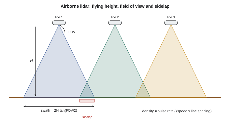
Swath, density and the flight plan

For a scanner with full field of view FOV flown at height \(H\) above ground, the swath width is

Adjacent lines are spaced at \(W(1 - q)\), where \(q\) is the sidelap, the fraction of a swath overlapped by its neighbour, commonly 20 to 50 percent. The number of pulses fired per second, the pulse repetition rate, is spread over the area the aircraft covers each second. With ground speed \(v\), the density from a single pass averaged over the swath is

and because overlap areas are covered twice, the aggregate density over the whole project is the pulse rate divided by the area covered per second of new ground, \(D = \text{PRR}/(v\,W(1-q))\). The nominal pulse spacing (NPS), the typical distance between pulses, is about \(1/\sqrt{D}\). These simple relations ignore the uneven distribution of points across the swath, the loss of pulses over water and dark surfaces, and the gain from multiple returns, but they are what every flight plan starts from.

import math
# Corridor flight plan: 24 km of canal, 2 km wide corridor
H = 1100.0        # flying height above ground, m
v = 65.0          # ground speed, m/s (about 126 knots)
fov = 40.0        # full field of view, degrees
prr = 800e3       # pulse repetition rate, pulses per second
sidelap = 0.30
width, length = 2000.0, 24000.0

swath = 2 * H * math.tan(math.radians(fov / 2))
density_single = prr / (v * swath)                      # pulses per m2, one pass
line = swath * (1 - sidelap)
lines = math.ceil((width - swath) / line) + 1
agg = density_single * swath / line                     # aggregate density with sidelap
print(f"swath {swath:.0f} m, line spacing {line:.0f} m, flight lines {lines}")
print(f"single-pass density {density_single:.1f} pulses/m2, NPS {1/math.sqrt(density_single):.2f} m")
print(f"aggregate density with {sidelap:.0%} sidelap {agg:.1f} pulses/m2, NPS {1/math.sqrt(agg):.2f} m")
t_line = length / v / 60
print(f"time on line {t_line:.1f} min each, {lines*t_line:.0f} min on lines in total")

# Footprint and the error a 0.005 deg boresight roll error causes at the swath edge
gamma = 0.25e-3
edge = H / math.cos(math.radians(fov / 2))
print(f"footprint at nadir {H*gamma*100:.0f} cm, at the edge {edge*gamma*100:.0f} cm")
dz = edge * math.radians(0.005) * math.sin(math.radians(fov / 2))
dx = edge * math.radians(0.005) * math.cos(math.radians(fov / 2))
print(f"0.005 deg roll error at the edge: {dx*100:.1f} cm across track, {dz*100:.1f} cm in height")

# Multiple pulses in the air: the range at which the next pulse leaves before the echo returns
mta = 299792458.0 / (2 * prr)
print(f"pulse interval range {mta:.0f} m -> at {edge:.0f} m slant range {math.floor(edge/mta)+1} pulses in the air")

# Flying height trades density against the number of lines
for h in (800.0, 1100.0, 1500.0):
    sw = 2 * h * math.tan(math.radians(fov / 2)); ln = sw * (1 - sidelap)
    d = prr / (v * ln)
    print(f"H {h:5.0f} m: swath {sw:4.0f} m, {math.ceil((width - sw) / ln) + 1} lines, aggregate {d:5.1f} pts/m2, NPS {1/math.sqrt(d):.2f} m")

swath 801 m, line spacing 561 m, flight lines 4
single-pass density 15.4 pulses/m2, NPS 0.26 m
aggregate density with 30% sidelap 22.0 pulses/m2, NPS 0.21 m
time on line 6.2 min each, 25 min on lines in total
footprint at nadir 28 cm, at the edge 29 cm
0.005 deg roll error at the edge: 9.6 cm across track, 3.5 cm in height
pulse interval range 187 m -> at 1171 m slant range 7 pulses in the air
H   800 m: swath  582 m, 5 lines, aggregate  30.2 pts/m2, NPS 0.18 m
H  1100 m: swath  801 m, 4 lines, aggregate  22.0 pts/m2, NPS 0.21 m
H  1500 m: swath 1092 m, 3 lines, aggregate  16.1 pts/m2, NPS 0.25 m

At 1,100 m above ground with a 40° field of view the swath is 801 m, lines are 561 m apart with 30 percent sidelap, and four lines cover the 2 km corridor. At 800,000 pulses per second and 65 m/s the aggregate density is about 22 pulses per square metre, a nominal pulse spacing of 0.21 m, comfortably denser than the specification. Each line takes six minutes, so the whole corridor needs about 25 minutes on line, plus turns and the transit from the airport. The table at the end shows the main lever the planner has: flying lower raises density but needs more lines; flying higher saves lines but costs density and footprint size.

The code also shows that at this pulse rate the pulses are only 187 m apart in range: the scanner fires about seven more pulses before the echo of the first returns from 1,171 m. Modern systems handle these multiple pulses in the air by tracking which echo belongs to which pulse, a problem called range ambiguity. It is solved by the system, but it can fail over steep terrain, where the range changes abruptly, producing points at a wrong range; the flying contractor's processing includes checks for such misassigned returns.

Specifications for airborne lidar

Specifications state what must be delivered: density, accuracy, classification, formats, coverage and reporting. Rather than writing their own, most agencies adopt a published base specification and add project requirements.

In Canada, Natural Resources Canada and Public Safety Canada publish the Federal Airborne LiDAR Data Acquisition Guideline, now at version 3.1 (2022), written for flood mapping but used widely. Its baseline level asks for an aggregate nominal pulse density of at least 2 pulses per square metre (spacing no more than 0.71 m), a non-vegetated vertical accuracy of 10 cm RMSE, a vegetated vertical accuracy of 30 cm at the 95th percentile, and limits on the agreement within and between swaths; appendices describe denser, more accurate levels for demanding uses. Provinces and municipalities have their own programs and specifications, and the national CanElevation series distributes many provincial and federal acquisitions. Ines specifies the guideline's baseline with a denser target of 8 pulses per square metre and 5 cm RMSE on the canal's hard surfaces, because the seepage study needs detailed bank geometry.

A good specification also covers the parts that are easy to forget: the coordinate reference system and its realization and epoch, the geoid model used to convert ellipsoidal heights, tile size and naming, the point cloud format and version (lesson 7), classification codes, the bare-earth model's cell size and treatment of water bodies and bridges, breaklines along water edges, metadata and the report. Each of these has caused disputes on someone's project.

Linear-mode, single-photon and drone lidar

The sensor described so far is a linear-mode system: each pulse is strong enough that its echo is detected as a waveform, giving one or several returns per pulse. Two other kinds of airborne lidar are common. Single-photon and Geiger-mode systems use weak pulses split into many beamlets and detectors sensitive enough to register single photons. They fly higher and faster and produce very dense data over large areas at low cost per square kilometre, but the raw data contain many noise points from sunlight that must be filtered statistically, and their behaviour in vegetation and on dark surfaces differs from linear-mode systems. Both kinds have been used for national programs.

At the other end of the scale, lidar on drones has become common for sites up to a few square kilometres. The physics and the georeferencing are the same, with lighter scanners, smaller IMUs and flying heights of 50 to 120 m, which give high density and small footprints but narrower swaths. Drone flights are governed by Transport Canada's rules in Part IX of the Canadian Aviation Regulations (GEOM-310), and the smaller IMU makes boresight calibration and strip adjustment even more important. The district's coulee monitoring in lesson 12 uses a drone lidar for one epoch.

Footprint, beam angle and terrain

At 1,100 m a 0.25 mrad beam has a footprint about 28 cm across at nadir, slightly larger at the swath edge. On sloping ground, and particularly on steep coulee banks, the footprint spreads along the slope and the echo broadens, so ranges become less precise and the effective position of the point less certain. The scan angle also matters: points near the swath edge see the ground obliquely, penetrate vegetation less well, and are more affected by errors in roll. Many specifications limit the usable scan angle, or the contractor trims the swath edges.

The code's boresight line shows why. An uncorrected roll misalignment of only 0.005° displaces points at the swath edge by about 10 cm across track and 3.5 cm in height, and it does so in opposite directions on lines flown in opposite directions. That pattern is the signature that lesson 10 uses to detect and correct the boresight.

Flying the survey

The flight is planned for a day with clear skies below the aircraft, light winds and, for a survey that must map ground under vegetation, a season with low foliage. In the district's prairie setting, the contractor aims for late autumn after harvest and before snow, or early spring after melt and before green-up; snow on the ground is unacceptable because the bare-earth surface would be the snow surface. Flights over the canal must also avoid the irrigation season, when the canal is full and the water surface hides the bed, unless the district can schedule a drawdown.

GNSS base stations operate throughout the flight, and the crew flies a cross line perpendicular to the main lines, crossing them all, which provides a check on the relative accuracy of the strips and helps estimate boresight errors. The contractor also flies the lines over a calibration site near the airport, with buildings and surveyed ground, at the start of the project. Grant's crew, meanwhile, surveys checkpoints on open, flat, hard ground and in each type of vegetation, spread through the corridor, never giving their coordinates to the contractor (lesson 10).