
GEOM-350 · Lesson 1 of 12 · 21 min
Lidar principles
Coulee Geomatics has a new kind of contract from the irrigation district. Marta Kowalchuk, the district's water manager, wants a three-dimensional record of the assets that matter most: the 1957 headworks gate structure on the Oldman River, the 24 km main canal and its access road, the coulee banks where InSAR showed slow movement, and the storage reservoir whose capacity has never been measured since it was filled. Ruth Albrecht, the principal, has asked Ines Dahl, the firm's lidar specialist, to lead the work with Leah Tran, who will run the quality control, Theo Martel, who will process the data, and Grant Okonkwo's field crew. Every product in this course, from the scan of a single pier to the airborne survey of the whole corridor, rests on one measurement: the distance from a laser to a surface. This lesson explains how that distance is measured and what limits it.
What lidar is
Lidar, short for light detection and ranging, measures distances by timing light. A laser emits a short pulse or a modulated beam, the light reflects from a surface, a detector records the echo, and the electronics convert the delay into a range. A scanning mechanism steers the beam so that thousands to millions of ranges are measured each second, each in a known direction. Range plus direction gives a point in the scanner's own coordinate system; adding the scanner's position and orientation in the world gives a point in project coordinates. A collection of such points is a point cloud. Unlike photogrammetry, which needs light from the sun and texture on the surface, lidar supplies its own light and measures range directly, so it works at night, on featureless surfaces such as fresh snow or smooth concrete, and, most importantly for mapping, through gaps in vegetation.
Three kinds of system are used in this course. A terrestrial laser scanner (TLS) sits on a tripod and sweeps the scene around it, producing millimetre-level detail of structures within tens to a few hundred metres. A mobile mapping system (MMS) carries one or more scanners on a vehicle, boat or backpack, with satellite positioning and an inertial measurement unit to track the platform as it moves. An airborne system (ALS) flies in an aircraft or, at smaller scale, on a drone, and maps the ground over kilometres in strips. The physics of ranging is the same in all three; what differs is the range, the platform's motion and how the scanner's position is known.
Ranging by time of flight
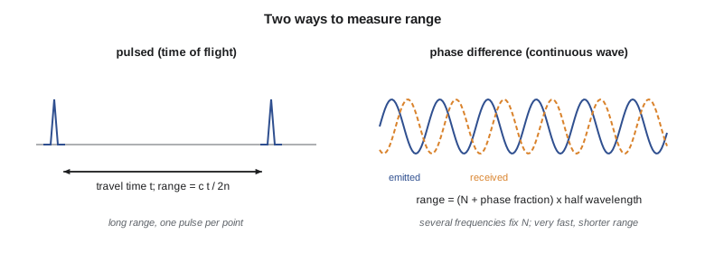
The simplest and most common method is pulsed time-of-flight ranging. The laser fires a pulse a few nanoseconds long, and a fast timer measures the interval \(t\) until the echo arrives. Light travels to the target and back, so the range is half the distance travelled:
where \(c\) is the speed of light in vacuum, 299,792,458 m/s, and \(n\) is the group refractive index of the air along the path. In air near the ground \(n\) is about 1.00027 for near-infrared light; it depends on temperature, pressure and, slightly, humidity, which is why precise instruments ask for, or measure, the weather. Ignoring it over 1,000 m makes ranges about 0.27 m too long, a large error for airborne mapping and one that the processing software removes routinely. For a terrestrial scanner at 30 m the effect is about 8 mm, still too large to ignore for structural work.
Timing must be extremely fine. Light covers 0.3 m in a nanosecond, so each nanosecond of timing error is 0.15 m of range. Modern receivers do not simply note when the echo crosses a threshold; they digitize the echo and find its centre by fitting a shape to it, which brings timing resolution to tens of picoseconds, a few millimetres of range. The detector, the pulse length and the electronics together set the range precision, typically 2 to 5 mm for terrestrial scanners at short range and 2 to 3 cm for airborne systems.
Ranging by phase difference
Some terrestrial scanners use continuous-wave phase ranging instead. The laser's intensity is modulated by a sine wave of frequency \(f\), and the instrument compares the phase of the returning light with the phase it sent. The phase difference gives the fraction of a cycle by which the echo lags; the range is
where \(\lambda_m\) is the modulation wavelength and \(N\) the unknown number of whole half-wavelengths. The phase tells the fraction precisely but says nothing about \(N\): a 100 MHz modulation repeats every 1.5 m of range, so a target at 87.456 m and one at 88.955 m give the same phase. Instruments resolve this by measuring with several frequencies at once. A coarse frequency with a long unambiguous range gives an approximate distance, good enough to fix \(N\) for the fine frequency, which supplies the precision. Phase scanners measure very quickly, up to about two million points per second, with low noise, but their range is limited to a few hundred metres at most and they are more sensitive to mixed returns at edges. Many current scanners use hybrid or waveform-digitizing designs that blur the old distinction, and manufacturers describe them in their own terms; the user's task is to read the specification for range, rate and noise rather than to classify the method.
import math
C0 = 299792458.0          # speed of light in vacuum, m/s
N_AIR = 1.00027           # group refractive index of air (typical, near-infrared)

def tof_range(t):
    """Range from a two-way travel time t (s)."""
    return C0 * t / (2.0 * N_AIR)

# 1. Pulse time of flight: an airborne return and a scanner return
for name, t in (("airborne, 1000 m class", 6.6713e-6), ("terrestrial wall", 2.0018e-7)):
    print(f"{name:24s} t = {t*1e9:9.2f} ns  range = {tof_range(t):9.3f} m")
dt = 1e-11
print(f"10 ps timing error -> {C0*dt/2*1000:.2f} mm of range")
print(f"refraction ignored at 1000 m -> {1000*(N_AIR-1)*1000:.0f} mm too long")

# 2. Phase ranging with two modulation frequencies
f_fine, f_coarse = 100e6, 1e6
lam = lambda f: C0 / (N_AIR * f)
U_fine, U_coarse = lam(f_fine) / 2, lam(f_coarse) / 2   # unambiguous ranges
true_r = 87.4562
phi_fine = (true_r / U_fine) % 1.0          # measured fractions of a cycle
phi_coarse = (true_r / U_coarse) % 1.0
coarse = phi_coarse * U_coarse
n = round((coarse - phi_fine * U_fine) / U_fine)
r = (n + phi_fine) * U_fine
print(f"unambiguous range: fine {U_fine:.3f} m, coarse {U_coarse:.1f} m")
print(f"coarse estimate {coarse:.3f} m, integer cycles n = {n}, range {r:.4f} m")

# 3. Footprint from beam divergence and the effect of incidence angle
gamma = 0.25e-3     # full-angle divergence, rad
for R in (10, 100, 1000):
    d = R * gamma
    print(f"range {R:5d} m: footprint {d*100:6.1f} cm, at 60 deg incidence {d/math.cos(math.radians(60))*100:6.1f} cm long")

# 4. Relative signal strength (extended target, lidar equation)
def power(R, rho=0.4, inc=0.0):
    return rho * math.cos(math.radians(inc)) / R**2
p0 = power(100)
for R, rho, inc in ((100, 0.4, 0), (200, 0.4, 0), (100, 0.1, 0), (100, 0.4, 70)):
print(f"R {R:3d} m, reflectance {rho:.1f}, incidence {inc:2d} deg: {power(R, rho, inc)/p0:6.3f} of reference")airborne, 1000 m class t = 6671.30 ns range = 999.733 m terrestrial wall t = 200.18 ns range = 29.998 m 10 ps timing error -> 1.50 mm of range refraction ignored at 1000 m -> 270 mm too long unambiguous range: fine 1.499 m, coarse 149.9 m coarse estimate 87.456 m, integer cycles n = 58, range 87.4562 m range 10 m: footprint 0.2 cm, at 60 deg incidence 0.5 cm long range 100 m: footprint 2.5 cm, at 60 deg incidence 5.0 cm long range 1000 m: footprint 25.0 cm, at 60 deg incidence 50.0 cm long R 100 m, reflectance 0.4, incidence 0 deg: 1.000 of reference R 200 m, reflectance 0.4, incidence 0 deg: 0.250 of reference R 100 m, reflectance 0.1, incidence 0 deg: 0.250 of reference R 100 m, reflectance 0.4, incidence 70 deg: 0.342 of reference
The code shows the numbers that matter in practice. A two-way travel time of 6.671 µs corresponds to an airborne range of about 999.7 m once refraction is included; a 10 picosecond timing error is 1.5 mm. The phase example recovers 87.4562 m by using the 1 MHz coarse measurement (150 m unambiguous range) to fix 58 whole cycles of the 100 MHz fine measurement. The footprint lines show why airborne points are not points at all: a 0.25 mrad beam is 25 cm wide at 1,000 m and twice as long on a slope inclined 60° to the beam.
The beam, its footprint and what it hits
A laser beam is not infinitely thin. It leaves the instrument with some diameter and spreads at a small angle called the beam divergence, usually quoted in milliradians as the full angle within which a stated fraction of the energy lies. At range \(R\) the footprint diameter is approximately
where \(d_0\) is the exit diameter and \(\gamma\) the divergence. For a terrestrial scanner with \(\gamma\) of a few tenths of a milliradian, the footprint at 10 m is a few millimetres; for an airborne system at 1,000 m it is tens of centimetres. Everything inside the footprint contributes to the echo. When the footprint falls across an edge, such as the corner of a pier or the top of a wall, part of the energy returns from the near surface and part from the far one, and the instrument may report a point between them that lies on neither: a mixed pixel, or edge effect. Such points appear as a fringe of false points in mid-air behind edges and must be filtered (lesson 6).
The angle at which the beam meets the surface, the incidence angle, matters too. A beam striking a surface obliquely spreads its footprint into an ellipse, lengthened by \(1/\cos\theta\), and returns less energy, so the range is noisier and may be biased. Scanning the downstream face of a dam from its toe, or a road surface from a vehicle at grazing angles, produces exactly these conditions. Good field planning keeps incidence angles below about 60° for important surfaces.
How strong is the echo?
The lidar equation describes the received power. For an extended target, one larger than the footprint, such as a wall or the ground, the received power falls with the square of range and is proportional to the surface's reflectance at the laser wavelength and to the cosine of the incidence angle:
where \(\rho\) is reflectance, \(\eta_{atm}\) the atmospheric transmission and \(\eta_{sys}\) the system efficiency. Doubling the range cuts the echo to a quarter; a dark surface with reflectance 0.1 returns a quarter as much as a light one with 0.4. Wet asphalt, dark roofing and fresh black plastic are notoriously poor targets in the near-infrared, while vegetation and dry concrete are bright. Water absorbs near-infrared light strongly and reflects it mainly where the surface faces the sensor, which is why near-infrared lidar shows lakes as holes in the data and why bathymetric systems use green light (lesson 11).
Most systems record the strength of each echo as an intensity value. Intensity is useful for interpretation, because paint markings, signs and wet patches stand out, and for classification, but it is not a calibrated reflectance unless the vendor has corrected it for range, incidence and gain. Comparing raw intensity between scanners, or even between flight lines, is risky.
One pulse, several returns
When the footprint meets a tree, part of the light reflects from leaves near the top, part from branches lower down, and the rest from the ground. A discrete-return system records the times of the strongest peaks in the echo, typically up to four or more returns per pulse, labelled first, intermediate and last. A full-waveform system digitizes the whole echo, often at a sample every nanosecond, and leaves the identification of peaks to processing. Multiple returns are the reason airborne lidar can map the ground under forest: even in a dense canopy some pulses reach the ground through gaps, and their last returns build a bare-earth surface that photogrammetry cannot see.
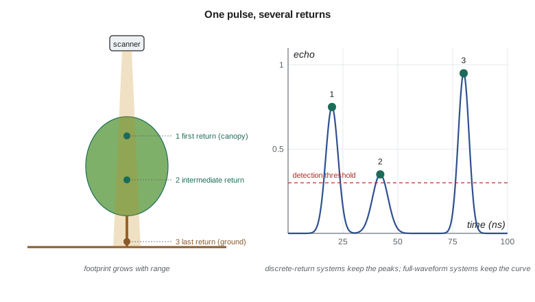
Two returns must be separated in time by at least the pulse width and the receiver's recovery time to be detected as separate. For a few-nanosecond pulse that is roughly 0.5 to 1.5 m of range, so a low shrub over the ground often produces one blended return that lies a little above the true ground: one reason why short vegetation is the hardest cover for lidar terrain mapping.
Wavelength and eye safety
Most topographic lidar works in the near-infrared, at about 905 nm, where inexpensive semiconductor lasers are available, or at 1,064 nm and 1,550 nm. Light at 1,550 nm is absorbed in the front of the eye and allows higher pulse energy for the same eye-safety class, which is one reason long-range scanners use it. Bathymetric systems add a green channel at 532 nm because green light penetrates clear water. Every laser product is classified by its accessible emission, from Class 1 (safe under all reasonably foreseeable conditions) through Classes 1M, 2, 2M, 3R and 3B to Class 4.
In Canada, laser products are regulated under the Radiation Emitting Devices Act, and classification follows the international standard IEC 60825-1. Most terrestrial and mobile scanners are Class 1 or 1M, but some long-range and airborne systems are Class 3R, 3B or 4, which brings controls set out in the operator's manual and the employer's occupational health and safety program: a nominal ocular hazard distance below the aircraft, warning notices, restricted viewing with binoculars or survey telescopes, and training. Ines makes reading the laser class part of every project's hazard assessment.
Viewing a Class 1M or 2M beam through magnifying optics can make it hazardous, a real risk when a survey crew sets up a total station beside an operating scanner. The rule on Coulee Geomatics sites is simple: nobody looks at a scanner through optics while it is running.
Lidar and photogrammetry compared
| Property | Lidar | Photogrammetry (lesson-level comparison) |
|---|---|---|
| Light source | Its own laser; works day or night | Sunlight or flash; needs good illumination |
| Measurement | Range and direction to each point | Image coordinates; depth from overlapping images |
| Texture needed | No | Yes; fails on uniform surfaces |
| Vegetation | Multiple returns reach the ground through gaps | Sees only the visible top surface |
| Colour and detail | Intensity only, unless cameras are added | Full colour, sharp edges and fine detail |
| Typical cost per area | Higher equipment cost | Lower equipment cost |
| Water | Near-infrared absorbed; green penetrates clear water | Surface glare; bottom only in very clear shallow water |
For the district's work the choice is rarely either-or. The airborne lidar system flown in lesson 4 carries a medium-format camera, the mobile mapping vehicle has six cameras that add colour to the points, and the terrestrial scanner photographs each setup. Lidar provides the geometry, cameras provide the colour and the interpretability, and the drone photogrammetry of GEOM-310 remains the cheaper choice for open stockpiles and bare construction sites.
Common mistakes
MistakeUsing a manufacturer's maximum range as the working range.
InsteadMaximum range is quoted for bright targets; dark, wet or oblique surfaces return much less.
MistakeTreating airborne lidar points as exact points.
InsteadEach is the average over a footprint tens of centimetres wide; edges and slopes blur.
MistakeComparing raw intensity values between scanners or flight lines.
InsteadIntensity depends on range, angle and gain; only corrected intensity is comparable.
MistakeIgnoring refraction and weather settings.
InsteadAt 1,000 m the refractive index of air changes range by about 0.27 m.
Summary and key terms
- Lidar measures range by timing light, and direction by the scanner's angle encoders; range plus direction gives a point.
- Pulsed time of flight uses R = ct/2n; phase ranging uses the phase of a modulated beam and several frequencies to fix the whole cycles.
- The beam footprint grows with range and with incidence angle; mixed returns at edges create false points.
- Echo strength falls with the square of range and depends on reflectance and incidence; near-infrared light is absorbed by water.
- Multiple returns and full-waveform recording let airborne lidar see the ground under vegetation.
- Laser class and eye-safety controls are part of every lidar project.
- Lidar
- Light detection and ranging: measuring distances by timing laser light.
- Time of flight
- Ranging by measuring the travel time of a laser pulse to the target and back.
- Phase ranging
- Ranging from the phase difference between emitted and received modulated light.
- Beam divergence
- The angle at which a laser beam spreads, setting the footprint size at a given range.
- Footprint
- The area on the target illuminated by one laser pulse.
- Multiple returns
- Separate echoes from one pulse that strikes several surfaces at different ranges.
- Full waveform
- Recording of the entire returned echo rather than only its peaks.
- Intensity
- A recorded measure of echo strength, useful for interpretation but not calibrated by default.
- Mixed pixel
- A false point at an edge, produced when one footprint strikes two surfaces.
Practice problems
Work each problem on paper first, then reveal the answer to check.
A pulse returns after 200.0 ns. What is the range, ignoring refraction?
Show answer
About 29.98 m.
What range error results from a 1 ns timing error?
Show answer
About 0.15 m.
A phase scanner modulates at 50 MHz. What is its unambiguous range for the fine measurement?
Show answer
About 3 m (half the 6 m modulation wavelength).
What is the footprint of a 0.3 mrad beam at 800 m?
Show answer
About 24 cm.
By what factor does the echo fall when range triples?
Show answer
By nine, to about 11 percent.
Lesson quiz · 5 questions
Score 60% or more to complete this lesson.
Create a free account to save your progress, take quizzes and earn a certificate.