Terrain analysis

The district's engineer had three questions about the land surface. Which coulees drain to each culvert under the canal embankment, and how large are their catchments, so that culverts due for replacement could be resized? Where are slopes steep enough along the canal banks to make erosion or sliding likely? And where does runoff from fields collect against the embankment, where ponding had been mistaken for seepage more than once? All three are terrain analysis questions, answered from a digital elevation model by computing slope, aspect, flow direction and flow accumulation and delineating catchments. This lesson describes elevation models and their sources, the standard terrain derivatives and how they are computed, hydrological analysis of a DEM, and the corrections that canals and culverts require.

Elevation models

A digital elevation model (DEM) represents the height of the land surface. The term is used loosely, so it helps to be precise. A digital terrain model (DTM) represents the bare ground, with vegetation and buildings removed. A digital surface model (DSM) represents the top of everything, including crops, trees and structures. Both are usually stored as rasters of regularly spaced heights. A triangulated irregular network (TIN) represents the surface by triangles joining irregularly spaced points, such as surveyed spot heights and breaklines along canal banks and road edges, with heights between points interpolated linearly within each triangle. A TIN can use many points where the terrain is complex and few where it is flat, and it honours breaklines exactly, which makes it the usual form for engineering design surfaces. Grids are simpler to analyse and are the usual form for regional terrain analysis.

The district's terrain data came from airborne lidar. The CanElevation series of Natural Resources Canada includes a high-resolution DEM, at 1 m or 2 m where lidar has been flown, derived from federal, provincial and municipal lidar projects, and coarser national elevation data elsewhere. The Alberta government has also acquired lidar across much of the province. For the service area, Theo used the 1 m bare-earth model, checked against 60 GNSS points on open, flat ground, where it agreed to about 0.1 m RMSE vertically, with heights in CGVD2013.

The accuracy of a DEM depends on the terrain and cover as well as the sensor. Lidar bare-earth models are most accurate on open, flat ground and less accurate under dense vegetation, on steep slopes and over water, where the lidar returns are poor and heights are interpolated. The canal itself appears in a lidar DEM as the water surface on the day of the flight, not the canal bed, and embankments appear as solid walls even where culverts pass through them. Both facts matter for hydrological analysis.

Slope and aspect

Slope is the steepness of the surface, the magnitude of its gradient, and aspect is the direction the slope faces, the compass direction of steepest descent. On a grid they are computed from the elevations of a 3 × 3 neighbourhood. Horn's method, used by most GIS software, estimates the east-west and north-south gradients as weighted differences across the window, giving double weight to the cells adjacent to the centre. With the window cells labelled a to i in rows from the north-west,

where \(\Delta\) is the cell size, and slope and aspect follow as

with the aspect measured clockwise from north. Slope may be reported in degrees or as a percentage, the tangent times 100; a 45° slope is 100 %. Aspect is undefined on flat ground and is usually coded as a special value there. Slope computed from a DEM depends strongly on cell size: a 30 m DEM smooths the steep banks of a coulee into gentle slopes that a 1 m DEM shows correctly. Curvature, the second derivative of the surface, distinguishes convex slopes, which shed water, from concave slopes and hollows, which collect it.

A hillshade is an image of the surface as if lit from a chosen direction, usually from the north-west at 45° above the horizon. Its brightness at each cell is the cosine of the angle between the light and the surface normal, computed from slope and aspect. Hillshades show terrain shape very effectively and are the usual backdrop for maps of the district, although they say nothing quantitative. Lighting from the north-west matches the way most readers perceive relief, and lighting from the south can make valleys look like ridges.

Flow direction and accumulation

Hydrological terrain analysis follows water downhill across the DEM. The D8 method, introduced by O'Callaghan and Mark in 1984, assigns each cell a single flow direction toward whichever of its eight neighbours gives the steepest descent, with diagonal distances taken as \(\sqrt{2}\) cells. Flow accumulation then counts, for each cell, how many cells drain through it, by passing each cell's count to its downstream neighbour in order from the highest cells to the lowest. Cells with large accumulation form the drainage network; the catchment of any point is the set of cells that drain to it. Methods that divide flow among several downslope neighbours, such as D-infinity, represent flow on smooth hillslopes better, while D8 is adequate for defining channels and catchments.

import math
# 10 m DEM of a coulee draining to a culvert under the lateral embankment (elevations in m)
z = [[912.4, 911.8, 911.0, 910.6, 911.1, 911.9, 912.6],
     [911.6, 910.7, 909.8, 909.2, 909.9, 910.8, 911.7],
     [910.9, 909.7, 908.5, 907.8, 908.6, 909.8, 910.9],
     [910.3, 908.9, 907.4, 906.5, 907.5, 908.9, 910.2],
     [909.8, 908.2, 906.6, 905.4, 906.7, 908.3, 909.7],
     [909.5, 907.9, 906.1, 904.6, 906.2, 908.0, 909.4],
     [909.3, 907.7, 905.9, 904.1, 905.9, 907.8, 909.2]]
c = 10.0; R, C = len(z), len(z[0])

def horn(r, k):        # slope (degrees) and aspect (degrees clockwise from north) by Horn's method
    a, b, cc = z[r - 1][k - 1], z[r - 1][k], z[r - 1][k + 1]
    d, f = z[r][k - 1], z[r][k + 1]
    g, h, i = z[r + 1][k - 1], z[r + 1][k], z[r + 1][k + 1]
    dzdx = ((cc + 2 * f + i) - (a + 2 * d + g)) / (8 * c)        # east positive
    dzdy = ((a + 2 * b + cc) - (g + 2 * h + i)) / (8 * c)        # north positive (row 0 is north)
    slope = math.degrees(math.atan(math.hypot(dzdx, dzdy)))
    aspect = (math.degrees(math.atan2(-dzdx, -dzdy)) + 360) % 360  # direction the slope faces (downhill)
    return slope, aspect, dzdx, dzdy
def hillshade(r, k, az=315.0, alt=45.0):
    s, asp, _, _ = horn(r, k)
    zen, sr, ar = math.radians(90 - alt), math.radians(s), math.radians(asp)
    v = math.cos(zen) * math.cos(sr) + math.sin(zen) * math.sin(sr) * math.cos(math.radians(az) - ar)
    return max(0, round(255 * v))
for r, k in ((2, 2), (3, 4), (4, 3)):
    s, a, gx, gy = horn(r, k)
    print(f"cell ({r},{k}): slope {s:4.1f} deg ({100 * math.tan(math.radians(s)):4.1f} %), aspect {a:5.1f} deg, hillshade {hillshade(r, k)}")

# D8 flow direction: each interior cell drains to the adjacent cell with the steepest drop
nbr = [(-1, -1), (-1, 0), (-1, 1), (0, -1), (0, 1), (1, -1), (1, 0), (1, 1)]
to = {}
for r in range(R):
    for k in range(C):
        best = None
        for dr, dk in nbr:
            rr, kk = r + dr, k + dk
            if 0 <= rr < R and 0 <= kk < C:
                drop = (z[r][k] - z[rr][kk]) / (c * math.hypot(dr, dk))
                if drop > 0 and (best is None or drop > best[0]): best = (drop, (rr, kk))
        if best: to[(r, k)] = best[1]
arrows = {(-1, -1): "↖", (-1, 0): "↑", (-1, 1): "↗", (0, -1): "←", (0, 1): "→", (1, -1): "↙", (1, 0): "↓", (1, 1): "↘"}
print("\nD8 flow directions (o = no lower adjacent cell: an outlet or pit)")
for r in range(R):
    print(" ".join(arrows[(to[(r, k)][0] - r, to[(r, k)][1] - k)] if (r, k) in to else "o" for k in range(C)))
# Flow accumulation: number of upstream cells draining through each cell (cells processed from high to low)
acc = {(r, k): 1 for r in range(R) for k in range(C)}
for cell in sorted(acc, key=lambda q: -z[q[0]][q[1]]):
    if cell in to: acc[to[cell]] += acc[cell]
print("\nflow accumulation (cells)")
for r in range(R): print(" ".join(f"{acc[(r, k)]:3d}" for k in range(C)))
out = (6, 3)
print(f"\ncatchment of the culvert at cell {out}: {acc[out]} cells = {acc[out] * c * c / 10000:.2f} ha within this DEM tile")

cell (2,2): slope  8.6 deg (15.1 %), aspect 140.4 deg, hillshade 152
cell (3,4): slope  8.8 deg (15.5 %), aspect 231.6 deg, hillshade 181
cell (4,3): slope  4.6 deg ( 8.0 %), aspect 183.6 deg, hillshade 170

D8 flow directions (o = no lower adjacent cell: an outlet or pit)
↘ ↘ ↘ ↓ ↙ ↙ ↙
↘ ↘ ↘ ↓ ↙ ↙ ↙
↘ ↘ ↘ ↓ ↙ ↙ ↙
↘ ↘ ↘ ↓ ↙ ↙ ↙
→ → ↘ ↓ ↙ ← ←
→ → → ↓ ← ← ←
→ → → o ← ← ←

flow accumulation (cells)
  1   1   1   1   1   1   1
  1   2   2   4   2   2   1
  1   2   3   9   3   2   1
  1   2   3  16   3   2   1
  1   3   6  23   6   3   1
  1   2   3  42   3   2   1
  1   2   3  49   3   2   1

catchment of the culvert at cell (6, 3): 49 cells = 0.49 ha within this DEM tile

The small DEM is a coulee whose floor runs south through column 3 to a culvert at the bottom edge. Slopes on its sides are about 15 %, with the west side facing south-east and the east side facing south-west, and the hillshade values show the north-west lighting: the west side, facing away from the light, is darker. The flow directions converge on the coulee floor, and accumulation grows down the floor to 49 cells at the culvert, the whole tile, since every cell in this small example drains there. On the full 1 m DEM the culvert's catchment was 186 ha, more than three times the area on the 1958 drawing, because a field drain installed in the 1980s had diverted a neighbouring coulee into this one. The culvert was resized accordingly.

Pits, embankments and culverts

Real DEMs contain pits, cells or groups of cells lower than all their neighbours, from which D8 has no outflow. Some are real, such as prairie potholes and sloughs, which are common in southern Alberta and Montana and genuinely store runoff; most are errors or small artefacts. Standard workflows fill pits to their spill point before computing flow directions, so that water can always leave. Filling every depression is wrong where real wetlands should hold water, so hydrologists often fill only small or shallow pits and treat larger depressions as storage.

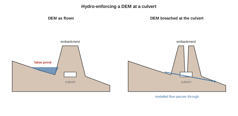
Linear features raise a bigger problem. A canal embankment or road fill in a lidar DEM is a continuous wall, and water modelled on the DEM ponds behind it or runs along it, even where a culvert carries the real water through. The fix, called hydro-enforcement or breaching, cuts a channel through the embankment in the DEM at each culvert, using the culvert locations from the GIS. Leah's first run without breaching produced catchments that ended at the embankment and ponds that did not exist; after breaching at the 260 surveyed culverts, the catchments matched the field drainage. The canal itself also needs care: water modelled on the DEM drains into the canal, which is correct for runoff in many places but must be checked, because the district's canal is designed not to take runoff, and in places it is protected by a berm on the uphill side.

Catchments and culvert sizing

A catchment (watershed) is delineated from flow directions by finding every cell whose flow path passes through the outlet, the culvert in this case. Its area, together with rainfall intensity and a runoff coefficient, gives the design flow by simple methods such as the rational method for small catchments, \(Q = CiA\), and the GIS also supplies the longest flow path and its slope for estimating the time of concentration. Leah produced a catchment for every culvert and attached its area, longest flow path and mean slope to the culvert record, so that the engineer could screen all 260 culverts for capacity in an afternoon and focus field checks on the ones that appeared undersized.

Visibility and volumes

Two other terrain analyses were useful to the district. A viewshed finds every cell visible from an observer point, by testing the line of sight to each cell against the DEM, and is used to place radio repeaters for the gate telemetry and cameras at structures; the district's new repeater on a coulee rim was sited after a viewshed showed it could see 9 of the 11 automated gates. Volume calculations compare two surfaces: a DEM before and after work gives the volume of excavation and fill, and a DEM of a reservoir basin gives its storage at each water level, the stage-storage curve used to operate it.