Overlay and buffer analysis

Two requests reached Leah in the same week. The first came from the district's agronomist: a map of the strip of land within 30 m of every lateral, where the district's operating rules restrict spraying of pesticides close to open water, with the area of each field inside the strip so that landowners could plan their spraying. The second came from the engineer: a map of seepage risk along the canal, combining soil permeability, depth to groundwater and distance from the canal, so that a drainage levy for a new interceptor drain could be shared among the fields that would benefit. Both requests are classic GIS analyses built from two operations, buffering and overlay. This lesson explains how they work in vector and raster form, the problems they produce and how results such as areas and shares should be computed and reported.

Buffers

A buffer is the zone within a specified distance of a feature. The buffer of a point is a circle; the buffer of a line is a corridor with rounded ends; the buffer of a polygon is the polygon enlarged outward, or shrunk if the distance is negative. Buffers may have a fixed distance or a distance taken from an attribute, such as a setback that depends on the size of the watercourse, and several distances may be combined into rings. When buffers of nearby features overlap, they can be kept separate, so each feature has its own zone, or dissolved into a single zone. Line ends may be rounded or flat, and corners rounded, mitred or bevelled; the rounded form is the true set of points within the distance, and the others are simplifications used where they match a legal or engineering definition.

Software builds a buffer from a line by offsetting each segment by the distance on both sides, joining the offsets around each vertex with arcs, and removing any loops created where the line bends sharply. Arcs are approximated by short segments, so a buffer's area is slightly smaller than the true value, by an amount that depends on the number of segments per quarter circle. For a single straight segment of length \(L\) buffered by a distance \(r\), the true area is

which is a useful check. Buffers must be computed in a projected CRS with units of length; a buffer of '30' in a geographic CRS is 30 degrees, and even a correctly scaled distance in degrees produces an ellipse rather than a circle because degrees of longitude are shorter than degrees of latitude.

Vector overlay

Overlay combines two or more layers to produce a new layer whose features carry the attributes of all the inputs where they coincide. The common operations differ in which parts of the inputs are kept. Intersect keeps only the areas common to both layers, with attributes from both. Union keeps all areas of both, split wherever their boundaries cross. Identity keeps all of the first layer, split by the second where they coincide. Erase (or difference) removes from the first layer the areas covered by the second. Clip cuts the first layer to the outline of the second without adding its attributes. Symmetrical difference keeps the areas covered by one layer or the other but not both.

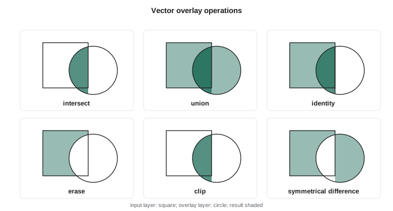
Overlay is computationally the heaviest common GIS operation. Every boundary of one layer must be tested against every boundary of the other for intersections, the boundaries split at those points, the resulting pieces assembled into new polygons and each polygon's attributes determined from the inputs. Spatial indexes make this feasible for large layers by testing only nearby boundaries. A simpler special case, clipping a polygon against a convex polygon, can be done edge by edge with the Sutherland-Hodgman algorithm, which the code below uses.

Slivers and tolerances

Overlaying two layers that represent the same boundary from different sources produces slivers: long, thin polygons along the boundary where the two versions disagree by small amounts. A field boundary digitized from an orthophoto and the same boundary from the parcel layer may differ by half a metre along its whole length, and overlaying them creates a sliver hundreds of metres long and less than a metre wide, with the attributes of one field and the wrong parcel. Slivers inflate polygon counts, distort statistics such as the number of fields in a zone, and are hard to see on a map. They are reduced by building layers from a common source where possible, snapping boundaries to one another within a cluster tolerance before overlay, and removing polygons below a minimum width or area afterwards, merging them with their largest neighbour. The tolerance should be chosen from the accuracy of the data, large enough to absorb their disagreement and small enough not to merge real features.

Attributes after overlay

When overlay splits a polygon, its attributes must be passed to the pieces, and how depends on what each attribute means. Categorical attributes, such as crop or soil class, apply to every piece unchanged. Extensive attributes, which are totals for the polygon such as an assessed levy, a population or a volume of water, must be divided among the pieces, usually in proportion to area. Intensive attributes, which are densities or rates such as yield per hectare or depth to water, apply to each piece unchanged and must be averaged with area weights, not summed, when pieces are combined. Area-weighted apportionment assumes the quantity is spread evenly within each original polygon, which is often only approximately true; dasymetric methods use an additional layer, such as irrigated land, to spread it more realistically.

import math
def area(p):
    return abs(sum(x1 * y2 - x2 * y1 for (x1, y1), (x2, y2) in zip(p, p[1:] + p[:1]))) / 2
def clip(subject, clipper):            # Sutherland-Hodgman: clipper must be convex and counter-clockwise
    out = subject
    for (ax, ay), (bx, by) in zip(clipper, clipper[1:] + clipper[:1]):
        inp, out = out, []
        if not inp: break
        side = lambda p: (bx - ax) * (p[1] - ay) - (by - ay) * (p[0] - ax) >= 0
        def meet(p, q):
            x1, y1 = p; x2, y2 = q
            d = (x2 - x1) * (by - ay) - (y2 - y1) * (bx - ax)
            t = ((ax - x1) * (by - ay) - (ay - y1) * (bx - ax)) / d
            return (x1 + t * (x2 - x1), y1 + t * (y2 - y1))
        for i, q in enumerate(inp):
            p = inp[i - 1]
            if side(q):
                if not side(p): out.append(meet(p, q))
                out.append(q)
            elif side(p): out.append(meet(p, q))
    return out
def buffer_segment(a, b, r, n=16):     # a segment buffered by r: two half circles joined by straight sides
    ang = math.atan2(b[1] - a[1], b[0] - a[0])
    pts = [(b[0] + r * math.cos(ang - math.pi / 2 + math.pi * k / n), b[1] + r * math.sin(ang - math.pi / 2 + math.pi * k / n)) for k in range(n + 1)]
    pts += [(a[0] + r * math.cos(ang + math.pi / 2 + math.pi * k / n), a[1] + r * math.sin(ang + math.pi / 2 + math.pi * k / n)) for k in range(n + 1)]
    return pts

# 1. A 30 m setback buffer around the reach of Lateral 7 from (800, 1000) to (1600, 900)
a, b, r = (800.0, 1000.0), (1600.0, 900.0), 30.0
buf = buffer_segment(a, b, r)
L = math.dist(a, b)
print(f"buffer area {area(buf):,.0f} m2 (polygon with 16 segments per end); exact 2rL + pi r2 = {2 * r * L + math.pi * r * r:,.0f} m2")

# 2. Clip the adjoining fields to the buffer: area of each field inside the spray setback
fields = {"7-13": [(800, 0), (1600, 0), (1600, 880), (800, 980)],
          "7-14": [(800, 1020), (1600, 920), (1600, 1700), (800, 1700)]}
for f, p in fields.items():
    part = clip(p, buf)
    print(f"field {f}: {area(p) / 10000:6.2f} ha, inside the 30 m setback {area(part) / 10000:5.2f} ha ({area(part) / area(p):.1%})")

# 3. Overlay with a seepage-risk zone and apportion a drainage levy of 12,000 levy units by area
risk = [(1100, 600), (1900, 600), (1900, 1300), (1100, 1300)]
more = {"7-16": [(1600, 0), (2400, 0), (2400, 680), (1600, 880)]}
parts = {f: area(clip(p, risk)) for f, p in {**fields, **more}.items()}
total = sum(parts.values())
print(f"\nseepage-risk zone {area(risk) / 10000:.2f} ha; fields inside it {total / 10000:.2f} ha (the rest is right-of-way and land outside these three fields)")
for f, x in parts.items():
    print(f"  {f}: {x / 10000:5.2f} ha in zone -> {12000 * x / total:7.0f} levy units")

# 4. A sliver: the same boundary from two sources, offset by 0.6 m over 800 m
v1 = [(800, 0), (1600, 0), (1600, 880), (800, 980)]
v2 = [(800.6, 0), (1600, 0), (1600, 880), (800.6, 980)]
print(f"\nsliver between versions: {area(v1) - area(v2):.0f} m2, a strip 0.6 m wide along the 980 m west boundary")

buffer area 51,183 m2 (polygon with 16 segments per end); exact 2rL + pi r2 = 51,201 m2
field 7-13:  74.40 ha, inside the 30 m setback  0.82 ha (1.1%)
field 7-14:  58.40 ha, inside the 30 m setback  0.82 ha (1.4%)

seepage-risk zone 56.00 ha; fields inside it 40.27 ha (the rest is right-of-way and land outside these three fields)
  7-13: 15.56 ha in zone ->    4637 levy units
  7-14: 17.44 ha in zone ->    5196 levy units
  7-16:  7.28 ha in zone ->    2168 levy units

sliver between versions: 558 m2, a strip 0.6 m wide along the 980 m west boundary

The buffer polygon with 16 segments per half circle is 18 m² smaller than the exact value, a negligible difference. Each field adjoining this reach of Lateral 7 has about 0.8 ha inside the 30 m setback, which is about 1 % of each field; the setback had looked much larger on the district's small-scale map, where the lateral's line symbol alone was wider than 30 m. The seepage-risk zone covers 56 ha, of which about 40 ha lies in the three fields, and the levy is shared in proportion to those areas. A 0.6 m disagreement along one 980 m boundary produces a sliver of more than 500 m², larger than many real features in the parcel layer.

Raster overlay and suitability

The seepage-risk map was easier to build in raster form. Leah reclassified three 10 m rasters onto a common scale of 1 (low) to 3 (high): soil permeability from the soil survey, depth to groundwater from the interpolated surface (Lesson 10), and distance from the canal, computed as a global distance operation from the canal cells. A weighted overlay then combined them cell by cell, with weights of 0.4 for depth to groundwater, 0.35 for permeability and 0.25 for distance, agreed with the engineer after reviewing the seepage reports. Cells with a weighted score above 2.4 were classed as high risk and converted to polygons for the levy calculation.

Raster overlay avoids slivers, because every layer is on the same grid, and is fast regardless of how complex the boundaries are. Its results are limited by the cell size, and the conversion of results back to polygons produces stair-stepped edges. Suitability and risk models of this kind are only as good as their scores and weights. Leah tested the result by changing each weight by 0.1 and checking how much of the high-risk area changed; the core of the zone along the coulee reach stayed the same in every case, which gave the board confidence, while the edges moved by up to 100 m, which was reported with the map. She also checked the zone against the seepage reports: 34 of the 41 reports in the previous five years fell in the high-risk class.

Multi-criteria analysis

Weighted overlay is the simplest form of multi-criteria decision analysis. More formal methods help stakeholders set weights consistently, such as the analytic hierarchy process, which derives weights from pairwise comparisons of the criteria, and fuzzy membership functions replace sharp class thresholds with gradual transitions, so that a depth to water of 1.9 m is not treated completely differently from 2.1 m. Whatever the method, the criteria, scores, weights and their sources should be documented and the result presented as one outcome of stated assumptions, not as a measurement.

Legal setbacks deserve particular care. Where a regulation or bylaw sets a distance from a watercourse, the GIS buffer should follow the regulation's definition of where the distance is measured from, which is often the top of bank or a high water mark rather than a centreline. The district's spray setback was its own operating rule, measured from the canal's water's edge, and Leah buffered the water's edge polygon, not the centreline, for the version used in landowner notices; the centreline version in the code is only an approximation.