Spatial interpolation

The seepage-risk overlay in Lesson 7 used a raster of depth to groundwater, but nobody had measured the groundwater everywhere. The district had a few dozen observation wells, some installed when the canal was built and some added during the rehabilitation, where a staff member measured the water level with a tape each month of the irrigation season. Turning those scattered measurements into a continuous surface is spatial interpolation: estimating values at unsampled locations from values at sampled ones. The same need arises for rainfall from gauges, soil properties from cores, elevations from survey points and crop yields from monitors. This lesson covers the main deterministic interpolation methods, how to choose between them and test them, and the ideas behind kriging, which GEOM-440 develops further.

Why interpolation works

Interpolation rests on the observation, often called Tobler's first law of geography, that near things are more related than distant things. Depth to groundwater 50 m from a well is likely to be similar to the depth at the well; 5 km away, the well says little. Every interpolation method is a way of turning that idea into weights for the known values, and the methods differ in how the weights depend on distance and arrangement, whether the surface passes exactly through the data, and whether the method also estimates its own uncertainty.

Interpolation is only as good as the sampling. The district's 38 wells were concentrated along the canal, where the problems were, with few in the fields between laterals and none in the coulees. Leah added the levels from the province's Groundwater Observation Well Network for three wells near the district and water well records with reported static levels from the province's water well database, which are single readings at the time of drilling and much less reliable. Every value was tagged with its source so that the less reliable values could be weighted or excluded.

Classifying methods

Interpolation methods can be classified in several ways. Exact methods reproduce the measured value at every data point; inexact (smoothing) methods do not, which is appropriate when measurements contain noise. Global methods fit one function to all the data, such as a trend surface; local methods estimate each location from nearby points only. Deterministic methods compute the estimate from a fixed formula, while geostatistical methods treat the variable as a random field and choose weights from a model of its spatial correlation, which also provides an estimate of the error. The commonest methods in practice are nearest neighbour, inverse distance weighting, triangulation, splines and kriging.

Nearest neighbour and Thiessen polygons

The simplest estimate takes the value of the nearest data point. The regions closest to each point are Thiessen (Voronoi) polygons, bounded by the perpendicular bisectors between neighbouring points, and the surface is constant within each polygon and jumps at their edges. Thiessen polygons are a long-standing way of weighting rain gauges by the area each represents, and they are useful for categorical data, but they produce an unrealistic stepped surface for continuous variables such as groundwater depth.

Inverse distance weighting

Inverse distance weighting (IDW) estimates each location as a weighted mean of the data values, with weights that decrease with distance:

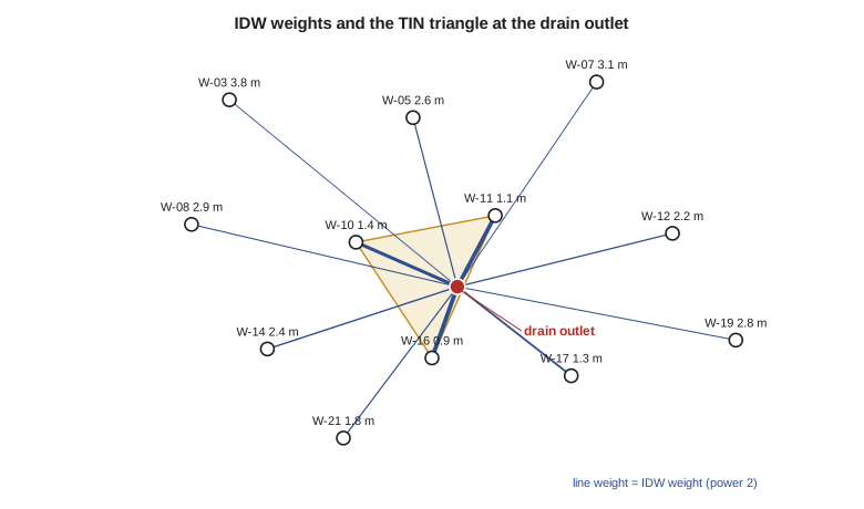
where \(d_i\) is the distance from the estimation point to data point \(i\) and \(p\) is the power, usually 2. A higher power gives more weight to the nearest points and produces a surface that approaches nearest neighbour; a lower power gives a smoother surface closer to the overall mean. The estimate is always between the lowest and highest data values, so IDW cannot predict a minimum or maximum that was not sampled, such as a hollow in the water table between wells. It also produces characteristic 'bull's-eyes' around isolated points. In practice the search is limited to the nearest few points or to a radius, which speeds computation and keeps distant points from influencing local estimates.

Triangulation

Triangulation connects the data points into a TIN, usually the Delaunay triangulation, in which no point lies inside the circumcircle of any triangle, which avoids long thin triangles where possible. The Delaunay triangulation is the dual of the Thiessen polygons: two points are joined by a triangle edge exactly when their Thiessen polygons share a boundary. Values inside each triangle are interpolated linearly from its three corners, with barycentric weights that sum to one. The surface is exact and continuous but has creases along triangle edges, and it is defined only within the convex hull of the data. Natural neighbour interpolation, devised by Robin Sibson, weights neighbours by how much of their Thiessen polygons a new point would take over, producing a smoother surface than linear triangulation with the same local behaviour.

Splines and trend surfaces

Splines fit a smooth surface through the data points by minimizing a measure of curvature, like a thin flexible sheet bent to pass through each point. Thin-plate splines produce very smooth surfaces and suit gently varying quantities such as water table elevations or climate normals; tension and regularized variants control how much the surface overshoots between points. Splines can predict values beyond the data range, which is both their strength, since a smooth surface may truly have a hollow between wells, and their weakness, since they can overshoot wildly where data are sparse. Trend surfaces fit a low-order polynomial in the coordinates to all the data by least squares. A first-order trend surface, a tilted plane, describes the regional slope of the water table toward the river; the residuals from it can then be interpolated locally.

import math
# Depth to groundwater (m below ground) at observation wells in July, district grid coordinates (m)
wells = {"W-03": (1200, 4100, 3.8), "W-05": (2650, 3900, 2.6), "W-07": (4100, 4300, 3.1), "W-08": (900, 2700, 2.9),
         "W-10": (2200, 2500, 1.4), "W-11": (3300, 2800, 1.1), "W-12": (4700, 2600, 2.2), "W-14": (1500, 1300, 2.4),
         "W-16": (2800, 1200, 0.9), "W-17": (3900, 1000, 1.3), "W-19": (5200, 1400, 2.8), "W-21": (2100, 300, 1.8)}
def idw(x, y, pts, p=2.0, exclude=None):
    num = den = 0.0
    for k, (xi, yi, zi) in pts.items():
        if k == exclude: continue
        d = math.hypot(x - xi, y - yi)
        if d < 1e-9: return zi
        w = 1.0 / d ** p; num += w * zi; den += w
    return num / den
def nearest(x, y, pts, exclude=None):
    return min((math.hypot(x - xi, y - yi), zi) for k, (xi, yi, zi) in pts.items() if k != exclude)[1]
site = (3000.0, 2000.0)                      # proposed interceptor drain outlet
print(f"estimates at {site}:")
print(f"  nearest well (Thiessen)  {nearest(*site, wells):.2f} m")
for p in (1, 2, 3):
    print(f"  IDW power {p}              {idw(*site, wells, p):.2f} m")

# Linear interpolation in a TIN triangle W-10, W-11, W-16 with barycentric weights
(x1, y1, z1), (x2, y2, z2), (x3, y3, z3) = wells["W-10"], wells["W-11"], wells["W-16"]
x, y = site
det = (y2 - y3) * (x1 - x3) + (x3 - x2) * (y1 - y3)
l1 = ((y2 - y3) * (x - x3) + (x3 - x2) * (y - y3)) / det
l2 = ((y3 - y1) * (x - x3) + (x1 - x3) * (y - y3)) / det
l3 = 1 - l1 - l2
print(f"  TIN (W-10, W-11, W-16)   {l1 * z1 + l2 * z2 + l3 * z3:.2f} m   weights {l1:.3f}, {l2:.3f}, {l3:.3f}")

# Leave-one-out cross-validation: predict each well from the others
print("\nleave-one-out cross-validation")
for name, f in (("nearest", lambda k: nearest(*wells[k][:2], wells, exclude=k)),
                ("IDW p=1", lambda k: idw(*wells[k][:2], wells, 1, exclude=k)),
                ("IDW p=2", lambda k: idw(*wells[k][:2], wells, 2, exclude=k)),
                ("IDW p=3", lambda k: idw(*wells[k][:2], wells, 3, exclude=k))):
    err = [f(k) - wells[k][2] for k in wells]
    print(f"  {name:8s} mean error {sum(err) / len(err):+.2f} m, RMSE {math.sqrt(sum(e * e for e in err) / len(err)):.2f} m, worst {max(err, key=abs):+.2f} m")

estimates at (3000.0, 2000.0):
  nearest well (Thiessen)  0.90 m
  IDW power 1              1.86 m
  IDW power 2              1.55 m
  IDW power 3              1.34 m
  TIN (W-10, W-11, W-16)   1.02 m   weights 0.050, 0.460, 0.491

leave-one-out cross-validation
  nearest  mean error -0.49 m, RMSE 0.81 m, worst -1.50 m
  IDW p=1  mean error -0.10 m, RMSE 0.88 m, worst -1.67 m
  IDW p=2  mean error -0.17 m, RMSE 0.83 m, worst -1.56 m
  IDW p=3  mean error -0.22 m, RMSE 0.79 m, worst -1.44 m

At the proposed drain outlet the estimates range from 0.90 m (nearest well, W-16) to 1.86 m (IDW with power 1). The TIN estimate, 1.02 m, uses only the three wells of the enclosing triangle, with W-10 contributing almost nothing because the outlet lies nearly on the edge between W-11 and W-16. The spread among methods, nearly a metre, is as large as the difference between a water table that threatens the embankment and one that does not, which shows why the choice of method needs testing rather than taste.

Testing an interpolation

Cross-validation tests an interpolation with the data themselves. In leave-one-out cross-validation, each data point is removed in turn, its value estimated from the others, and the error recorded. The mean error shows bias; the root mean square error shows typical accuracy; maps of the errors show where the method does badly. In the code, the four methods have similar RMSEs of about 0.8 m, and all underestimate on average, because the wells with the deepest water are on the edges of the network, where estimates are pulled toward the shallower interior. IDW with power 3 is slightly best by RMSE, but the differences are small compared with the errors themselves, which says more about the sparse network than about the methods. Leah's recommendation was to add six wells in the gaps between laterals before the next season, not to fine-tune the method.

Interpolating the right variable

The variable to interpolate is not always the one wanted. Depth to groundwater depends on both the water table and the ground surface, which varies sharply across coulees and embankments, so interpolating depths directly smears the terrain's shape into the result. Groundwater hydrologists therefore interpolate the water table elevation, which varies smoothly, and subtract it from the DEM to obtain depth. Leah did this for the final surface, using the 10 m DEM from Lesson 9: depth was shallow along the canal and in the coulee bottoms and deep under the higher fields, a pattern the direct interpolation of depths had missed. Areas where the interpolated water table rose above the DEM surface pointed either to springs, which the field crew confirmed at two locations, or to errors in the interpolation.

Kriging in brief

Kriging, named after the South African mining engineer Danie Krige and formalized by Georges Matheron, chooses the weights from a model of how similarity between values decreases with distance. The model is the semivariogram, which plots half the mean squared difference between pairs of values against the distance between them. It typically rises from a small value at short distances, the nugget, which reflects measurement error and variation at scales shorter than the sample spacing, to a plateau, the sill, at a distance called the range, beyond which values are unrelated. Given a fitted semivariogram, kriging solves for the weights that give the best linear unbiased estimate, and it also gives the kriging variance at every location, a map of uncertainty that depends on the arrangement of the data. Kriging can also use secondary variables, such as distance from the canal, that are known everywhere. The statistics of semivariogram fitting and the variants of kriging are covered in GEOM-440; here the essential point is that kriging is a statistical model whose assumptions should be checked, not a superior button.

Presenting interpolated surfaces

An interpolated surface looks equally certain everywhere, and readers take it that way unless told otherwise. Good practice is to show the data points on the map, to mask or shade areas far from any data, to report the cross-validation error and the method, and, where kriging is used, to map the kriging standard error alongside the estimate. The district's seepage map showed the wells as symbols and faded the surface beyond 1.5 km from the nearest well, so that the board could see where the map rested on measurements and where it was extrapolation.