
GEOM-330 · Lesson 5 of 12 · 24 min
Data capture and quality
With the data model agreed, the district's layers had to be filled. Some data would come from Grant's crew walking the laterals with GNSS receivers, some from digitizing the orthophotos made for the photogrammetry project, some from scanning and georeferencing the old as-built drawings, and some from converting the spreadsheet of water users and the CAD drawing of the main canal. Every source had its own errors, and the district needed to know how good the result was before anyone relied on it to dispatch a crew or bill a water user. This lesson covers the main methods of data capture, the conversion of legacy records, the elements by which data quality is described and measured, and the metadata that carry that description with the data.
Primary and secondary capture
Primary data capture measures the world directly: a GNSS survey of turnouts and culverts, a total station survey of a structure, a lidar flight, satellite imagery, a field inspection recorded on a tablet. Secondary capture derives data from existing sources: digitizing features from orthophotos or scanned maps, converting CAD drawings, keying coordinates from survey plans, loading public datasets and geocoding addresses. Primary capture is usually more accurate and current but more expensive; secondary capture is cheaper but inherits the age, scale and errors of its sources. Most projects combine both, using primary capture for the features that matter most and secondary sources for the rest.
Grant's crew surveyed every turnout, check, drop and culvert on the laterals with RTK GNSS, recording the structure type, size and condition on a tablet form at the same time, so that position and attributes were captured together. A crew could record about 40 structures a day on an accessible lateral, so the 420 turnouts and 260 culverts took about four weeks. The canal centreline itself was digitized from the orthophotos, which were accurate to a few decimetres, rather than walked, because a line digitized from an orthophoto was both cheaper and accurate enough for network analysis.
Digitizing and vectorization
On-screen digitizing traces features over a georeferenced image or map. Its accuracy depends on the source's accuracy, the display scale at which the operator works and the operator's care. Snapping, which moves a new vertex onto an existing vertex or line within a tolerance, prevents the gaps and overshoots that spoil topology. Digitizing at too small a display scale places vertices inaccurately; digitizing at too large a scale wastes time adding vertices that the source cannot support. Semi-automatic vectorization traces lines in scanned drawings or images automatically and leaves the operator to correct the result, which can be fast on clean drawings and slow on old, stained ones. Machine learning models now extract buildings, roads and field boundaries from imagery at scale, but their outputs still need checking against the requirements of the data model.
Georeferencing scanned drawings
The 1958 as-built drawings of the laterals showed structures that had since been buried, abandoned or forgotten, and they were the only record of some pipe sizes and inverts. Theo scanned them at 300 dots per inch and georeferenced each sheet by identifying control points, features visible on both the scan and the ground (structure corners, section corners, road intersections) whose ground coordinates were known from the GNSS survey. A transformation is then fitted from scan coordinates to ground coordinates. A similarity transformation (four parameters: two shifts, a scale and a rotation) preserves shape; an affine transformation (six parameters) also allows different scales in the two directions and a shear, which absorbs the uneven shrinkage of an old drawing; polynomial and rubber-sheeting transformations bend the image further to fit many points, at the risk of distorting areas between them.
With more control points than parameters, the transformation is fitted by least squares, as in the adjustment course, and the residuals at the control points show how well it fits. The root mean square (RMS) of the residuals is often reported as the accuracy of the georeferencing, but it measures fit to the points used, not accuracy elsewhere. Independent check points, not used in the fit, measure accuracy. A point with a much larger residual than the others usually signals a misidentified feature and should be investigated, not simply removed.
import math
def T(A): return [list(r) for r in zip(*A)]
def mul(A, B): return [[sum(a * b for a, b in zip(r, c)) for c in zip(*B)] for r in A]
def inv(A):
    n = len(A); M = [list(map(float, r)) + [1.0 if i == j else 0.0 for j in range(n)] for i, r in enumerate(A)]
    for c in range(n):
        p = max(range(c, n), key=lambda r: abs(M[r][c])); M[c], M[p] = M[p], M[c]
        d = M[c][c]; M[c] = [x / d for x in M[c]]
        for r in range(n):
            if r != c:
                f = M[r][c]; M[r] = [x - f * y for x, y in zip(M[r], M[c])]
    return [r[n:] for r in M]
def diag(v): return [[v[i] if i == j else 0.0 for j in range(len(v))] for i in range(len(v))]
def col(v): return [[x] for x in v]
# Georeferencing a scanned 1958 as-built plan: control points measured on the scan (pixels) and their
# ground coordinates from the GNSS survey (district grid, m). Affine model: E = a0 + a1 c + a2 r, N = b0 + b1 c + b2 r
gcp = [  # (column, row) on the scan -> (E, N)
    ((412.0, 388.0),   (5073.08, 8174.84)),
    ((3896.0, 455.0),  (5780.79, 8178.69)),
    ((3851.0, 2930.0), (5784.35, 7675.26)),
    ((455.0, 2874.0),  (5094.96, 7669.68)),
    ((2140.0, 1660.0), (5430.46, 7924.97)),
    ((1307.0, 2402.0), (5265.39, 7769.78)),
]
A = [[1.0, c, r] for (c, r), _ in gcp]
At = T(A); N = inv(mul(At, A))
pe = mul(N, mul(At, col([e for _, (e, n) in gcp])))
pn = mul(N, mul(At, col([n for _, (e, n) in gcp])))
a0, a1, a2 = (v[0] for v in pe); b0, b1, b2 = (v[0] for v in pn)
print(f"pixel size {math.hypot(a1, b1):.4f} m along rows, {math.hypot(a2, b2):.4f} m down columns, rotation {math.degrees(math.atan2(b1, a1)):.2f} deg")
ss = 0.0
for i, ((c, r), (e, n)) in enumerate(gcp, 1):
    de = a0 + a1 * c + a2 * r - e; dn = b0 + b1 * c + b2 * r - n
    ss += de * de + dn * dn
    print(f"GCP {i}: residual E {de:+.2f} m, N {dn:+.2f} m")
dof = 2 * len(gcp) - 6
print(f"RMS residual {math.sqrt(ss / len(gcp)):.2f} m; standard error of unit weight {math.sqrt(ss / dof):.2f} m ({dof} redundant observations)")

# Positional accuracy of turnouts digitized from the georeferenced plan, against independent GNSS check points
check = [  # (GIS E, GIS N, GNSS E, GNSS N)
    (5102.4, 8011.9, 5103.6, 8010.8), (5310.8, 7955.2, 5309.9, 7957.0), (5588.1, 7880.6, 5589.9, 7879.1),
    (5701.5, 7712.0, 5700.2, 7711.3), (5822.9, 7604.4, 5824.0, 7606.1), (5190.3, 7702.8, 5188.6, 7703.9),
    (5402.7, 7590.1, 5403.9, 7588.4), (5655.4, 7533.6, 5654.0, 7534.9), (5876.2, 7980.7, 5877.3, 7979.4),
    (5044.9, 7598.2, 5043.7, 7597.0),
]
dx = [g - s for g, _, s, _ in check]; dy = [g - s for _, g, _, s in check]
rx = math.sqrt(sum(d * d for d in dx) / len(dx)); ry = math.sqrt(sum(d * d for d in dy) / len(dy))
rr = math.hypot(rx, ry)
print(f"\nmean error E {sum(dx) / len(dx):+.2f} m, N {sum(dy) / len(dy):+.2f} m")
print(f"RMSE E {rx:.2f} m, N {ry:.2f} m, horizontal {rr:.2f} m")
print(f"NSSDA horizontal accuracy at 95 % = 1.7308 x RMSEr = {1.7308 * rr:.2f} m")

# Completeness: turnouts found by the field crew compared with those in the GIS for Lateral 7
field_crew = {f"7-{k}" for k in range(1, 23)} | {"7-14A"}
gis = {f"7-{k}" for k in range(1, 23) if k != 9} | {"7-23"}
print(f"\nomitted from GIS: {sorted(field_crew - gis)}; in GIS but not found (commission): {sorted(gis - field_crew)}")
print(f"completeness {len(field_crew & gis) / len(field_crew):.1%}")pixel size 0.2030 m along rows, 0.2034 m down columns, rotation 1.41 deg GCP 1: residual E +0.09 m, N +0.01 m GCP 2: residual E -0.12 m, N +0.00 m GCP 3: residual E +0.10 m, N +0.01 m GCP 4: residual E -0.09 m, N -0.05 m GCP 5: residual E +0.08 m, N -0.07 m GCP 6: residual E -0.05 m, N +0.09 m RMS residual 0.10 m; standard error of unit weight 0.10 m (6 redundant observations) mean error E +0.01 m, N +0.16 m RMSE E 1.32 m, N 1.38 m, horizontal 1.91 m NSSDA horizontal accuracy at 95 % = 1.7308 x RMSEr = 3.30 m omitted from GIS: ['7-14A', '7-9']; in GIS but not found (commission): ['7-23'] completeness 91.3%
The affine fit gives a pixel size of about 0.203 m in both directions, consistent with a 1:2,400 drawing scanned at 300 dots per inch, a rotation of 1.4° and residuals of about a decimetre. Yet the turnouts digitized from the georeferenced plan are, on average, 1.9 m from their GNSS positions, with a 95 % accuracy of 3.3 m. The plan fits its control points well, but it shows where the structures were designed, drawn at a scale where a pen line is half a metre wide, and some were built a metre or two from the plan. The georeferenced scans were therefore used for attributes, pipe sizes, inverts and dates, while positions came from the GNSS survey.
Legal descriptions and the survey grid
Land in the prairie provinces is described by the Dominion Land Survey, known in Alberta as the Alberta Township System (ATS). Townships about 6 miles square are numbered north from the 49th parallel and ranges west from a meridian; Lethbridge lies in townships 8 and 9, ranges 21 and 22, west of the fourth meridian (W4M). Each township has 36 sections of about one square mile (259 ha), numbered from 1 in the south-east corner, westward along the bottom row and back and forth to 36 in the north-east. Each section has four quarter sections of about 64.7 ha, and sixteen legal subdivisions (LSDs) of about 16.2 ha numbered the same way. A water user's land might be described as NE-22-9-22-W4, the north-east quarter of section 22, township 9, range 22, west of the fourth meridian, and a well as 12-22-9-22-W4, in LSD 12 of the same section.
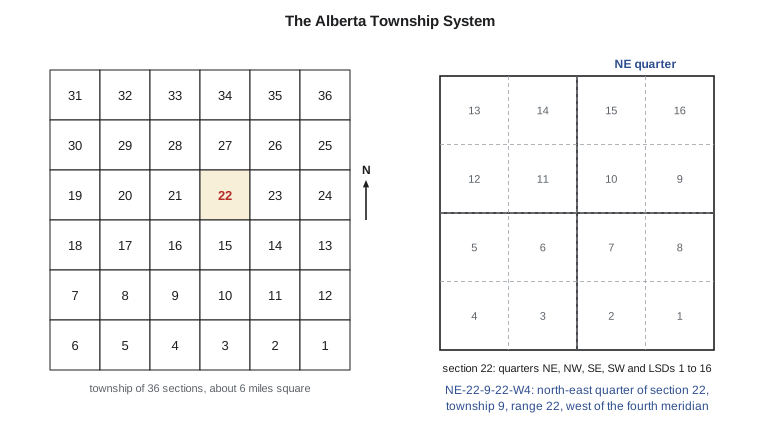
Converting legal descriptions into geometry is a form of geocoding: each description is parsed and matched to the corresponding polygon in the survey grid layer. Legal descriptions in a spreadsheet are rarely typed consistently, with variations in order, spacing and abbreviations, so Theo wrote a parser that normalized them, matched them against the grid and produced a list of the descriptions it could not match for a person to resolve. Of 1,240 descriptions, 1,176 matched automatically, 51 were corrected by hand and 13 referred to land that had since been subdivided, which needed the current parcel layer to resolve. Street addresses are geocoded the same way, against a reference layer of address points or road segments with address ranges, and the result should carry a match score so that poor matches can be reviewed.
Elements of data quality
The international standard ISO 19157 groups data quality into elements that apply to any geographic dataset. Each element can be measured, and the results reported in the metadata.
| Element | Question | Example measure for the district |
|---|---|---|
| Completeness | Is everything that should be there present, and nothing extra? | Percentage of turnouts found in the field that are in the GIS (omission) and GIS turnouts not found (commission) |
| Logical consistency | Does the data obey the model's rules? | Number of topology errors: dangles, overlapping fields, turnouts not on a lateral, invalid domain values |
| Positional accuracy | How close are positions to the truth? | RMSE against independent GNSS check points |
| Thematic accuracy | Are attributes and classes correct? | Percentage of culverts whose recorded diameter matches a field measurement; error matrix for crop classes |
| Temporal quality | Are data current and are dates correct? | Date of last verification of each structure; lag between a field change and its entry |
| Usability | Is the data fit for a stated use? | Statement that the network supports downstream tracing and dispatch |
Lineage, the history of a dataset's sources and processing steps, is not itself a quality element in the standard but is essential to judging quality: two layers with the same RMSE may differ greatly in how far they can be trusted if one was surveyed last year and the other digitized from a 1958 drawing.
Measuring positional accuracy
Positional accuracy is measured by comparing coordinates in the dataset with coordinates of the same points from an independent source of higher accuracy, at least three times better by common practice. The errors in each coordinate give the root mean square errors
and the mean errors reveal any systematic shift, such as a datum mix-up. The National Standard for Spatial Data Accuracy (NSSDA), published by the U.S. Federal Geographic Data Committee in 1998 and widely used in both countries, reports horizontal accuracy at 95 % confidence as 1.7308 times the radial RMSE when the errors in the two coordinates are similar and normally distributed, and asks for at least 20 well-distributed check points. The ASPRS standards discussed in the photogrammetry course now report RMSE directly. Whichever is used, the statement should say how many check points were used, how they were distributed and what source they came from.
Worked problem
Positional accuracy statement
Ten turnouts digitized from the scanned plan were compared with GNSS positions. The RMSE was 1.32 m in easting and 1.38 m in northing, and the mean errors were close to zero. What is the horizontal accuracy at 95 % confidence?
Show solution
- \[\mathrm{RMSE}_r = \sqrt{1.32^2 + 1.38^2} = 1.91 \text{ m}\]
- \[\text{Accuracy}_{95} = 1.7308 \times 1.91 = 3.30 \text{ m}\]
Answer: The digitized positions would be reported as tested to 3.3 m horizontal accuracy at 95 % confidence, with the caveat that ten points are fewer than the twenty the standard recommends. Because the mean errors are near zero, there is no sign of a systematic shift.
Checking and cleaning
Quality control is built into capture, not added at the end. Domains and constraints reject invalid attribute values as they are entered. Topology rules are validated after every editing session, and the errors are listed for correction: the district's first validation of the converted CAD network found 312 dangles, 41 duplicate lines and 17 places where laterals crossed without a junction. Attribute checks compare related values: a 600 mm culvert on a lateral with a design capacity that needs 1,200 mm deserves a field visit. Completeness is checked by sampling, as in the code, where the field crew found two turnouts missing from the GIS for Lateral 7 (one of them the unofficial 7-14A) and one in the GIS that no longer existed. Each check produces a list of issues with an owner and a resolution, so that cleaning is tracked rather than done once and forgotten.
Metadata
Metadata are data about data: what a dataset contains, who made it, from what sources, when, in what coordinate reference system, with what accuracy and under what terms it may be used. Without metadata, a dataset found on a shared drive five years later is of unknown value and is either trusted blindly or recreated at great cost. The ISO 19115 standard defines the content of geographic metadata, and ISO 19157 the reporting of quality within it.
In Canada, federal geospatial data follow the North American Profile of ISO 19115 and the federal government's open data metadata requirements, and Alberta's open data portal publishes metadata with each dataset. Leah wrote a short metadata record for each district layer covering its purpose, sources, capture dates, CRS, accuracy, attribute definitions, update procedure and contact, and stored it in the database alongside the data, so that it travelled with every export.
Common mistakes
MistakeReporting the georeferencing RMS as the accuracy of a scanned map.
InsteadMeasure accuracy with independent check points not used in the fit.
MistakeDeleting a control point with a large residual without investigation.
InsteadFind out why: a misidentified feature, a typing error or a real map distortion.
MistakeDigitizing at a display scale far smaller than the source.
InsteadWork at a scale where the source's detail is resolved, with snapping on.
MistakeTreating a dataset as complete because it has no topology errors.
InsteadCheck completeness separately against the field or another source.
MistakePublishing a layer without metadata.
InsteadRecord sources, dates, CRS, accuracy, definitions and contact with every layer.
Summary and key terms
- Primary capture measures directly; secondary capture derives from existing sources and inherits their limitations.
- Digitizing accuracy depends on the source, the display scale and snapping; automated extraction still needs checking.
- Scanned drawings are georeferenced by fitting a transformation to control points; residuals measure fit, check points measure accuracy.
- Legal descriptions in the survey grid are geocoded by parsing and matching, with unmatched records resolved by hand.
- ISO 19157 describes quality by completeness, logical consistency, positional, thematic and temporal accuracy, and usability.
- Positional accuracy is reported from RMSE against independent, more accurate check points.
- Metadata record what a dataset is, where it came from, how good it is and how it may be used.
- Primary data capture
- Measuring features directly in the field or by remote sensing.
- Control point
- A point identifiable on an image and with known ground coordinates.
- Check point
- An independent point used to measure accuracy, not to fit a transformation.
- Affine transformation
- A six-parameter linear transformation allowing shifts, rotation, two scales and shear.
- Geocoding
- Converting descriptions such as addresses or legal descriptions into locations.
- Completeness
- The degree to which all intended features, and no others, are present.
- Lineage
- The record of a dataset's sources and processing steps.
- Metadata
- Structured information describing a dataset.
Practice problems
Work each problem on paper first, then reveal the answer to check.
An RMSE of 0.80 m in x and 0.60 m in y. What is the NSSDA horizontal accuracy at 95 %?
Show answer
RMSEr = 1.00 m; accuracy = 1.73 m.
How many parameters does an affine transformation have, and how many control points are needed at minimum?
Show answer
Six parameters; three control points (six coordinates).
The field crew found 48 culverts; 45 are in the GIS, which also lists 2 culverts not found. What are the omission and commission counts?
Show answer
3 omitted, 2 committed; completeness 45/48 = 93.8 %.
Why should check points be at least three times more accurate than the data being tested?
Show answer
So that their own errors do not significantly inflate the measured RMSE.
In which section and quarter is land described as SW-10-9-22-W4?
Show answer
The south-west quarter of section 10 of that township and range.
Lesson quiz · 5 questions
Score 60% or more to complete this lesson.
Create a free account to save your progress, take quizzes and earn a certificate.