
GEOM-330 · Lesson 1 of 12 · 27 min
What a GIS is
By the end of the remote sensing program the irrigation district had crop maps, water use estimates, bank movement time series and change alerts, but they lived in folders on Theo Martel's workstation at Coulee Geomatics. Everything else the district knew was scattered further. The canal and its structures existed as 1950s and 1960s as-built drawings on linen and mylar, a CAD drawing of the main canal made for the rehabilitation project, and a binder kept by each ditch rider. The water users were rows in a spreadsheet, keyed by name, with land described by quarter section. Water orders were taken by phone and written into a daybook. When a culvert washed out under a range road in May, nobody could say quickly which turnouts were downstream of it, which landowners to call or when the culvert had last been replaced. Marta Kowalchuk, the district's water manager, asked Ruth Albrecht for a geographic information system that would bring all of this together. Ruth gave the design to Leah Tran, who had led the remote sensing analysis, with Theo on databases and scripts and Grant Okonkwo's crew on field data capture. This course follows that project from the first interviews to the web map the district's staff and water users now use every day.
A working definition
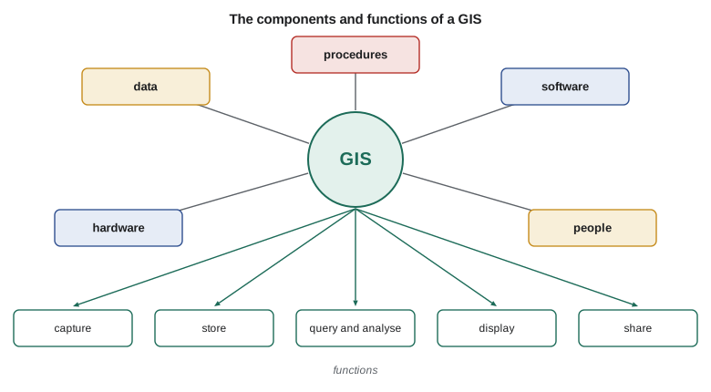
A geographic information system is an organized combination of data, software, hardware, people and procedures for capturing, storing, checking, analysing and displaying information that is referenced to locations on the Earth. The definition has two halves. The first half is the list of components: a GIS is not a program you install but a system that an organization runs. The second half is the list of functions, and it is the reason a GIS is more than a map. Every record in a GIS carries a location, so records can be related to one another by where they are, not only by what they say. A turnout can be found because it lies on Lateral 7, a field because it contains the turnout, a water user because they own the field, and a culvert because it lies upstream on the same lateral. None of those links has to be typed in by hand; they follow from geometry.
Each component matters. Data are the most expensive and longest-lived part: studies of GIS projects have long found that building and maintaining data costs far more than software and hardware combined, and the district's canal data will outlive any software it buys. Software provides the data structures and the tools. Hardware now ranges from servers and desktop workstations to tablets in a ditch rider's truck and GNSS receivers on a survey pole. People include the analysts who build the system and the staff who use it, and procedures are the rules that keep the data trustworthy: who may edit the canal network, how a new turnout is surveyed and entered, how often the parcel layer is refreshed and how errors are reported. Most failed GIS projects fail on the last two components, not the first three.
How a GIS differs from related tools
A GIS overlaps several other kinds of software, and the district already had some of them. Computer-aided design (CAD) software draws precise geometry, and the canal rehabilitation drawings were made in it. A CAD drawing, however, usually stores lines on layers with little attached information, and it is drawn in a local coordinate system for one project. A GIS stores each feature with attributes in tables, places all data in a common coordinate reference system and can answer questions across many datasets. A database management system stores and queries records very well but has no notion of geometry unless it is extended with spatial types, which is exactly what a spatial database does (Lesson 4). Remote sensing software, used in the previous course, processes images; its products become layers in a GIS. Building information modelling (BIM) describes structures in three dimensions in great detail, and asset management software tracks inspections, work orders and costs. In practice the district's GIS would exchange data with all of these: CAD for design, the remote sensing products for monitoring, and a maintenance system for work orders.
Questions a GIS answers
Geographers have long grouped the questions a GIS can answer into a few kinds. Questions of location ask what is at a place: which field contains this turnout, who owns the land at this point? Questions of condition ask where something is true: where are fields that grew alfalfa and lie within 200 m of the canal? Questions of trend ask what has changed: which turnouts were added since 2015, and where has the irrigated area grown? Questions of pattern ask whether there is structure: are seepage reports clustered along certain reaches? Questions of modelling ask what would happen: if check 4 is closed for repair, which turnouts lose water, and for how long can they be served from the reservoir? A useful exercise at the start of any project is to write down the questions the users actually ask, because they determine the data needed.
Leah spent two weeks interviewing district staff, the board chair, two ditch riders and a few water users. She asked each person what they needed to know, how often, how quickly and with what accuracy, and what they did today without a GIS. The answers sorted into a short list of products.
| User | Typical question | Layers needed | Accuracy and timeliness |
|---|---|---|---|
| Water manager | Which turnouts are downstream of a closed gate, and who must be called? | Canal network, structures, turnouts, fields, water users | Topologically correct; current within a day |
| Ditch riders | Where is turnout 7-14, and what was ordered for it today? | Turnouts, roads, orders | Positions to a few metres; orders live |
| Maintenance foreman | Which culverts are past their service life, and what is the shortest route to them? | Culverts with install year and condition, road network | Positions to a few metres; condition yearly |
| Board | How much area is irrigated by crop, and how has it changed? | Fields, crop map, water use | Areas to a few per cent; seasonal |
| Engineer | Where is the water table shallow near the canal, and where is seepage likely? | Wells, terrain, soils, seepage reports | Surface accuracy to tenths of a metre; yearly |
| Water users | Where are my turnouts and what did I use this season? | Own fields, turnouts, deliveries | Private to each user; seasonal |
Representing the world: objects and fields
Before any data are captured, a designer decides how each part of the world will be represented. Two views run through the whole subject. In the object view the world is made of discrete things with boundaries and identities: a turnout, a culvert, a field, a parcel of land, a road segment. Objects are naturally stored as vector features (Lesson 2), points, lines and polygons with attributes. In the field view the world is a set of quantities that vary continuously over space: elevation, depth to groundwater, soil moisture, crop water use. Fields are naturally stored as rasters (Lesson 3), regular grids of cells, or as surfaces such as triangulated networks. Many phenomena can be seen either way. Soils are mapped as polygons with a dominant soil type, but soil properties vary continuously within them. The canal is a line on a district map and an area on a large-scale plan. The choice depends on the questions, the scale and the data available.
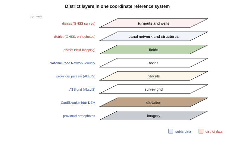
A GIS organizes data as layers or feature classes, each holding one kind of feature: the canal centreline, the structures, the turnouts, the fields, the parcels, the roads, the wells, the elevation model. Layers in the same coordinate reference system can be overlaid, queried together and drawn together. A good layer holds features of one geometry type with one set of attributes and a clear definition of what is and is not included. A layer called 'structures' that mixes gates, culverts, bridges and fence lines, half of them as points and half as lines, is a common inheritance from CAD and one of the first things to fix.
Scale, resolution and generalization
Map scale is the ratio of a distance on a map to the corresponding distance on the ground. A 1:50,000 map shows 1 mm on paper for 50 m on the ground. Large-scale maps (1:500, 1:1,000) show small areas in detail; small-scale maps (1:250,000, 1:1,000,000) show large areas with little detail. In a GIS, data can be drawn at any scale on screen, so the scale of a dataset really refers to the scale at which it was captured, which limits its positional accuracy and detail. A road digitized from a 1:250,000 map may be 100 m from the real road, and zooming in does not make it more accurate. This is why every layer needs a statement of its source, scale or resolution and accuracy, recorded in its metadata.
Generalization is the simplification of detail as scale decreases: features are selected or omitted, lines smoothed and simplified, small polygons merged and nearby features displaced so they remain legible. A district-wide map at 1:100,000 cannot show every turnout, and the canal drawn at true width would be thinner than a hair. Lesson 11 returns to generalization as a cartographic operation; here the point is that the capture scale should match the most detailed use. The district wanted to locate turnouts to a few metres, so their positions had to come from GNSS survey or large-scale orthophotos, not from a small-scale topographic map.
Georeferencing and coordinate reference systems
Every layer in a GIS must say how its coordinates relate to the Earth. That statement is its coordinate reference system (CRS). A geographic CRS gives latitude and longitude on an ellipsoid tied to a datum, as described in the geodesy course. A projected CRS transforms latitude and longitude into planar easting and northing in metres or feet using a map projection, so that distances and areas can be computed with ordinary plane geometry over a limited region. GEOM-340 covers projections in depth. For a GIS user the essential rules are few. Know the CRS of every dataset. Keep the master data in one projected CRS chosen for the region. Transform data correctly when they arrive in another CRS, including any datum transformation, rather than shifting them by eye until they line up. Software can reproject on the fly for display, but analysis such as buffering and area calculation should be done in an appropriate projected CRS.
For the district, Leah chose NAD83(CSRS) with UTM zone 12 north coordinates for the master data, matching the control survey and the provincial base data, with heights in CGVD2013. Many Alberta datasets also use the Alberta 3TM projection with a central meridian of 114° W; those would be transformed on loading. Coordinate reference systems are identified in software by codes from the EPSG registry, maintained by the geodesy subcommittee of the International Association of Oil and Gas Producers. Two codes appear constantly in practice: EPSG:4326 for latitude and longitude on WGS 84, used by GNSS receivers and most web data, and EPSG:3857 for the Web Mercator projection used by web map tiles (Lesson 12). Treating NAD83(CSRS) and WGS 84 coordinates as identical introduces errors of the order of a metre or more in western Canada, which is small on a regional map but matters for turnouts surveyed to a few centimetres.
Latitude and longitude are angles, not distances, and one of the commonest mistakes in GIS work is to compute distances or areas directly in degrees. A degree of latitude is about 111 km everywhere, but a degree of longitude shrinks with the cosine of latitude. Treating degrees as a square grid at the district's latitude overstates east-west distances by half or more. The code below compares the great-circle distance, a local equirectangular approximation and the naive calculation for distances across the service area, and converts a distance measured on a paper map.
import math
R = 6371000.0          # mean Earth radius, m
pts = {                # (latitude, longitude) in decimal degrees, NAD83(CSRS)
    "headworks":       (49.5851, -112.9553),
    "check 4":         (49.6327, -112.8710),
    "district office": (49.6942, -112.8418),
}
def haversine(a, b):
    p1, l1 = map(math.radians, a); p2, l2 = map(math.radians, b)
    h = math.sin((p2 - p1) / 2) ** 2 + math.cos(p1) * math.cos(p2) * math.sin((l2 - l1) / 2) ** 2
    return 2 * R * math.asin(math.sqrt(h))
def flat(a, b):         # naive: treat degrees as if they were a square grid
    return math.hypot(b[0] - a[0], b[1] - a[1]) * math.pi / 180 * R
def local(a, b):        # equirectangular: shrink longitude by cos(latitude)
    pm = math.radians((a[0] + b[0]) / 2)
    dx = math.radians(b[1] - a[1]) * math.cos(pm) * R
    dy = math.radians(b[0] - a[0]) * R
    return math.hypot(dx, dy)
for x, y in (("headworks", "check 4"), ("headworks", "district office")):
    a, b = pts[x], pts[y]
    g, f, e = haversine(a, b), flat(a, b), local(a, b)
    print(f"{x} -> {y}: great circle {g:8.1f} m, local {e:8.1f} m, naive degrees {f:8.1f} m ({100 * (f - g) / g:+.0f} %)")
# A distance measured on a printed map at 1:50,000
mm = 223.0
print(f"\n{mm:.0f} mm on a 1:50,000 map = {mm * 50000 / 1000:.0f} m on the ground")
print(f"one degree of longitude here = {math.radians(1) * math.cos(math.radians(49.64)) * R / 1000:.1f} km, one degree of latitude = {math.radians(1) * R / 1000:.1f} km")headworks -> check 4: great circle 8056.7 m, local 8056.7 m, naive degrees 10764.8 m (+34 %) headworks -> district office: great circle 14627.7 m, local 14627.7 m, naive degrees 17505.7 m (+20 %) 223 mm on a 1:50,000 map = 11150 m on the ground one degree of longitude here = 72.0 km, one degree of latitude = 111.2 km
Over 8 to 15 km the local approximation agrees with the great-circle distance to well under a metre, while the naive calculation is 20 to 34 % too long, depending on direction. A projected CRS removes the problem entirely for analysis within the region, which is one reason the master data are kept in UTM coordinates.
Worked problem
Map scale and ground distance
Grant measured 223 mm along a straight range road on a 1:50,000 topographic map. What is the ground distance, and what positional accuracy can be expected from features digitized from that map if the map was drawn to within 0.5 mm?
Show solution
- \[d = 223 \text{ mm} \times 50\,000 = 11\,150\,000 \text{ mm} = 11.15 \text{ km}\]
- \[\sigma \approx 0.5 \text{ mm} \times 50\,000 = 25 \text{ m}\]
Answer: The road is about 11.2 km long, and features digitized from the map are good to a few tens of metres at best, before any error from the digitizing itself. That is fine for a regional base map and far too coarse for turnouts.
Data the district did not have to create
A large part of any GIS comes from other organizations. Governments publish base data for roads, hydrography, boundaries, elevation and imagery, much of it free, and a district should use them wherever they meet its needs rather than redrawing what already exists. The skill is to know what is available, how current and accurate it is, and under what licence it may be used and shared.
In Canada the federal Open Government Portal and its Open Maps collection publish national datasets under the Open Government Licence – Canada. Natural Resources Canada's CanVec provides topographic vector data (roads, hydrography, buildings, land cover and more) compiled for scales from 1:50,000 and smaller, and CanElevation provides elevation models, including high-resolution lidar models where they exist. Alberta's provincial base data, such as the Alberta Township System grid, survey framework and parcel fabric, are distributed through AltaLIS on behalf of the province, some freely and some under licence, and the provincial open data portal publishes many other datasets. Municipal districts and counties maintain their own road and address data.
Leah built a data inventory listing, for each candidate layer, its source, date, scale or resolution, CRS, accuracy, licence and the district's use for it. Two decisions came out of it. Base layers such as roads, hydrography and the survey grid would be loaded from public sources and refreshed on a schedule, with the district never editing its own copies. Layers that only the district could know, the canal network, structures, turnouts, fields, water users and orders, would be built and maintained by the district, and these became the core of the project.
People, procedures and professional practice
A GIS for an organization of the district's size needs at least one person who owns it: someone responsible for the data model, the editing rules, backups and the publication of maps and services. The district decided to train one of its office staff, with Coulee Geomatics providing support under contract. Leah wrote procedures for the most common edits, a new turnout, a replaced culvert, a change of landowner, each describing who records the change, what evidence is needed and how it is checked. Without such rules, the data begin to drift within months of the project's end.
Work that defines property boundaries or establishes survey control is regulated: in Alberta, land surveys are made by Alberta Land Surveyors, and geomatics engineering is practised under the oversight of APEGA. A GIS parcel layer is an index to land titles, not a survey, and its lines should never be used to set a fence. Many GIS practitioners hold the voluntary GIS Professional certification offered by the GIS Certification Institute, and professional associations such as the Canadian Institute of Geomatics publish codes of ethics that apply to GIS work.
Software is the least lasting choice, but it shapes daily work. The district chose open-source desktop software, QGIS, for most staff, with a commercial desktop licence for the analyst who exchanges data with the provincial or state agencies and engineering firms, and an open-source spatial database, PostgreSQL with the PostGIS extension, as the shared store. Both desktop programs read and write the same open formats and connect to the same database, so the choice could be changed later without rebuilding the data. The open-source GDAL library underlies format conversion in most GIS software, including both desktop programs.
Common mistakes
MistakeComputing distances or areas directly in latitude and longitude.
InsteadUse a projected CRS, or geodesic formulas, for measurement.
MistakeAssuming two datasets share a CRS because they overlap on screen.
InsteadCheck the CRS of every dataset; on-the-fly reprojection can hide a datum error of a metre or more.
MistakeZooming in and treating small-scale data as precise.
InsteadRecord and respect the capture scale and accuracy of each layer.
MistakeStarting with software and screens.
InsteadStart with users' questions, then the data and procedures needed to answer them.
MistakeUsing a GIS parcel layer as a boundary survey.
InsteadParcel layers index ownership; boundaries are defined by legal surveys.
Summary and key terms
- A GIS combines data, software, hardware, people and procedures to capture, store, analyse and display located information.
- Location lets records be related by where they are, which distinguishes a GIS from CAD, ordinary databases and image processing software.
- GIS questions concern location, condition, trend, pattern and modelling; the users' questions determine the data needed.
- Discrete objects suit vector data; continuous fields suit rasters and surfaces.
- The capture scale and accuracy of a layer limit its use, however far one zooms in.
- Every layer needs a known coordinate reference system; analysis should be done in a suitable projected CRS.
- Public base data should be reused; data only the organization knows form the core of its GIS.
- Geographic information system
- An organized system of data, software, hardware, people and procedures for handling located information.
- Object view
- A representation of the world as discrete features with boundaries and identities.
- Field view
- A representation of the world as quantities varying continuously over space.
- Layer
- A collection of features of one kind and geometry type in one coordinate reference system.
- Map scale
- The ratio of a distance on a map to the corresponding ground distance.
- Generalization
- The simplification of detail for display or capture at smaller scales.
- Coordinate reference system
- The definition that relates a dataset's coordinates to locations on the Earth.
- EPSG code
- A numeric identifier for a coordinate reference system in the EPSG registry.
Practice problems
Work each problem on paper first, then reveal the answer to check.
A line measures 38 mm on a 1:250,000 map. What is the ground length?
Show answer
38 × 250,000 mm = 9.5 km.
Name the five components of a GIS and say which usually costs the most over the life of a system.
Show answer
Data, software, hardware, people and procedures; data usually cost the most.
Is depth to groundwater better treated in the object view or the field view? Why?
Show answer
The field view: it varies continuously across the area.
At latitude 49.6°, how long is one degree of longitude, taking R = 6,371 km?
Show answer
111.2 km × cos 49.6° = 72.1 km.
Classify the question 'Have seepage reports increased along the north reach since 2018?'
Show answer
A question of trend (and possibly pattern).
Lesson quiz · 5 questions
Score 60% or more to complete this lesson.
Create a free account to save your progress, take quizzes and earn a certificate.