
GEOM-330 · Lesson 6 of 12 · 20 min
Spatial queries
Once the layers were loaded and checked, the district's staff began asking questions of them, and most questions turned out to be queries: select the features that meet some conditions and report or map them. Some conditions were about attributes, such as all culverts installed before 1970. Others were about location, such as all fields within 200 m of Lateral 7, or the culvert nearest to a washout reported by a landowner. The most useful combined both, such as alfalfa fields within 200 m of the lateral, whose owners had to be told before the lateral was drained for repair. This lesson covers attribute queries, the spatial relationships on which spatial queries are built, distance and nearest-neighbour queries, and the spatial join, which transfers attributes from one layer to another by location.
Attribute queries
An attribute query selects features by conditions on their attributes, using comparison operators (equal, less than, greater than), set membership, text patterns and null tests, combined with the Boolean operators AND, OR and NOT. In SQL it is the WHERE clause of a SELECT statement, and in desktop GIS software it is often called 'select by attributes'. The result is a selection, a subset of features that can be mapped, counted, exported or used as the input to another query. Boolean logic needs care. 'Culverts in poor condition OR installed before 1970 AND on Lateral 7' is ambiguous unless parentheses say whether the lateral condition applies to both. Null values need care too: a culvert with an unknown installation year is neither before nor after 1970, and a query for 'not before 1970' does not return it.
Attribute queries also depend on the attribute's measurement scale. Equality tests suit nominal codes such as crop type. Range tests suit ratio values such as area or diameter. Text patterns are fragile when values have not been controlled by a domain: a query for 'alfalfa' misses 'Alfalfa' and 'alfalfa/grass' unless the data were cleaned or the query allows for them. That is one more reason to use domains at capture (Lesson 4).
Spatial relationships
Spatial queries select features by their geometric relationship to other features. The relationships are defined precisely in the Simple Features standard through the dimensionally extended nine-intersection model (DE-9IM). Each geometry is considered to have an interior, a boundary and an exterior. For a polygon, the interior is the area inside, the boundary its ring and the exterior everything outside; for a line, the boundary is its two end points and the interior the rest of the line; a point has only an interior. The relationship between two geometries is described by the dimension of the intersection of each part of one with each part of the other, a 3 × 3 matrix whose entries are empty, 0 (points), 1 (lines) or 2 (areas). Named predicates correspond to patterns in the matrix.
| Predicate | Meaning | District example |
|---|---|---|
| Intersects | The geometries share at least one point | Fields that the proposed pipeline route crosses or touches |
| Disjoint | No point in common (the opposite of intersects) | Wells that are nowhere near the right-of-way |
| Contains / Within | One geometry lies entirely inside the other, with interiors meeting | Turnouts within the district boundary; the field that contains a well |
| Touches | Boundaries meet but interiors do not | Fields that share a boundary with field 7-14 |
| Crosses | A line passes through the interior of another geometry, the intersection being of lower dimension | Roads that cross Lateral 7 |
| Overlaps | Geometries of the same dimension share some but not all interior | Fields that overlap the flood extent mapped in June |
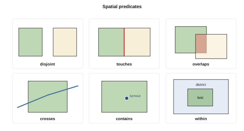
Some predicates surprise new users. A polygon does not contain a point on its own boundary, because containment requires the point to be in the interior; the predicate 'covers' includes boundary points. Two fields that share a boundary touch but do not overlap, which is exactly what a clean topological dataset should show; if a query reports that adjacent fields overlap, the data have sliver overlaps. A line that ends exactly on another line touches it but does not cross it. The exact meanings matter in automated checks. The district's rule 'every turnout must lie on a lateral' was implemented as 'the distance from the turnout to the nearest lateral is less than 0.5 m', not as an intersection, because surveyed points almost never fall exactly on a digitized line.
Distance and nearest-neighbour queries
Distance queries select features within a given distance of other features: fields within 200 m of a lateral, wells within 1 km of a reported seepage. They can be answered by buffering the target and testing intersection (Lesson 7), but spatial databases answer them directly with a distance-within function that uses the spatial index to find candidates and computes exact distances only for them. The distance between two geometries is the smallest distance between any of their points. For a polygon and a line it is zero if they intersect; otherwise it is found among the distances from the vertices of each to the segments of the other.
Nearest-neighbour queries ask for the closest feature, or the k closest features, to a location: the culvert nearest a washout, the three nearest observation wells to a new monitoring site. A naive search computes all distances and sorts them; spatial indexes support nearest-neighbour search directly by visiting index nodes in order of their distance from the query point. Straight-line distance is not always the right measure. The nearest culvert in a straight line may be on the other side of the canal, and the crew needs the nearest one they can reach by road, which is a network question (Lesson 8).
Spatial joins
A spatial join attaches attributes from one layer to features in another on the basis of their spatial relationship, as an ordinary join does on the basis of matching keys. Each well can be given the number of the field that contains it; each field can be given the count of seepage reports within it, or the mean depth to groundwater at the wells inside it; each turnout can be given the name of the nearest lateral. Joins may be one-to-one, taking a single matching feature, or one-to-many, producing a row for each match or summarizing the matches with counts, sums or means. A spatial join is how data captured independently, such as seepage reports phoned in by landowners and recorded as points, become usable alongside the district's own layers.
import math
fields = {  # field number: (crop, polygon in district grid, m); a 40 m right-of-way separates fields from the lateral
    "7-11": ("alfalfa", [(0, 0), (800, 0), (800, 980), (0, 980)]),
    "7-12": ("wheat",   [(0, 1020), (800, 1020), (800, 1800), (0, 1800)]),
    "7-13": ("alfalfa", [(800, 0), (1600, 0), (1600, 880), (800, 980)]),
    "7-14": ("canola",  [(800, 1020), (1600, 920), (1600, 1700), (800, 1700)]),
    "7-16": ("alfalfa", [(1600, 0), (2400, 0), (2400, 680), (1600, 880)]),
    "7-17": ("alfalfa", [(1750, 1150), (2400, 1150), (2400, 1900), (1750, 1900)]),
    "7-18": ("barley",  [(2500, 880), (3100, 880), (3100, 1500), (2500, 1500)]),
}
lateral7 = [(0, 1000), (800, 1000), (1600, 900), (2400, 700), (3000, 700)]
culverts = {"C-31": (400, 1000), "C-32": (1180, 952), "C-33": (2010, 798), "C-34": (2700, 700)}
reports = [(310, 940), (520, 955), (1420, 860), (1475, 870), (1530, 852), (1890, 760), (2150, 1220), (620, 1080)]

def area(p):
    return abs(sum(x1 * y2 - x2 * y1 for (x1, y1), (x2, y2) in zip(p, p[1:] + p[:1]))) / 2
def inside(pt, poly):
    x, y = pt; c = False
    for (x1, y1), (x2, y2) in zip(poly, poly[-1:] + poly[:-1]):
        if (y1 > y) != (y2 > y) and x < x1 + (y - y1) * (x2 - x1) / (y2 - y1): c = not c
    return c
def seg_dist(p, a, b):
    dx, dy = b[0] - a[0], b[1] - a[1]
    t = max(0.0, min(1.0, ((p[0] - a[0]) * dx + (p[1] - a[1]) * dy) / (dx * dx + dy * dy)))
    return math.hypot(p[0] - a[0] - t * dx, p[1] - a[1] - t * dy)
def cross(a, b, c, d):          # do segments ab and cd intersect?
    o = lambda p, q, r: (q[0] - p[0]) * (r[1] - p[1]) - (q[1] - p[1]) * (r[0] - p[0])
    return o(a, b, c) * o(a, b, d) <= 0 and o(c, d, a) * o(c, d, b) <= 0
def poly_line_dist(poly, line):
    ring = list(zip(poly, poly[1:] + poly[:1])); segs = list(zip(line, line[1:]))
    if any(cross(a, b, c, d) for a, b in ring for c, d in segs) or inside(line[0], poly): return 0.0
    return min(min(seg_dist(v, c, d) for v in poly for c, d in segs), min(seg_dist(v, a, b) for v in line for a, b in ring))

print("1. attribute query: alfalfa fields larger than 50 ha")
print("  ", [f for f, (crop, p) in fields.items() if crop == "alfalfa" and area(p) / 10000 > 50])
print("2. spatial query: fields within 200 m of Lateral 7 (0 = the lateral crosses or touches the field)")
for f, (crop, p) in fields.items():
    d = poly_line_dist(p, lateral7)
    if d <= 200: print(f"   {f} {crop:8s} distance {d:6.1f} m")
print("3. combined: alfalfa fields within 200 m of Lateral 7 ->",
      [f for f, (crop, p) in fields.items() if crop == "alfalfa" and poly_line_dist(p, lateral7) <= 200])
w = (1560.0, 905.0)
near = sorted((math.hypot(w[0] - x, w[1] - y), c) for c, (x, y) in culverts.items())
print(f"4. nearest culverts to the washout at {w}: " + ", ".join(f"{c} ({d:.0f} m)" for d, c in near[:2]))
print("5. spatial join: seepage reports counted in each field")
count = {f: 0 for f in fields}
for pt in reports:
    for f, (crop, p) in fields.items():
        if inside(pt, p): count[f] += 1
print(" ", ", ".join(f"{f}: {n}" for f, n in count.items() if n))1. attribute query: alfalfa fields larger than 50 ha ['7-11', '7-13', '7-16'] 2. spatial query: fields within 200 m of Lateral 7 (0 = the lateral crosses or touches the field) 7-11 alfalfa distance 19.8 m 7-12 wheat distance 20.0 m 7-13 alfalfa distance 19.4 m 7-14 canola distance 19.8 m 7-16 alfalfa distance 19.4 m 7-18 barley distance 180.0 m 3. combined: alfalfa fields within 200 m of Lateral 7 -> ['7-11', '7-13', '7-16'] 4. nearest culverts to the washout at (1560.0, 905.0): C-32 (383 m), C-33 (463 m) 5. spatial join: seepage reports counted in each field 7-11: 2, 7-12: 1, 7-13: 3, 7-16: 1, 7-17: 1
The attribute query finds three alfalfa fields over 50 ha. The distance query finds the five fields along Lateral 7, all about 20 m away because the right-of-way separates them from the centreline, and field 7-18 at 180 m; field 7-17 lies further back and is excluded. Combining the two gives the three alfalfa fields whose owners were notified before the lateral was drained. The nearest culvert to the washout is C-32, 383 m away in a straight line. The spatial join counts three seepage reports in field 7-13, more than in any other field, which pointed the engineer to the reach of Lateral 7 alongside it. One report, at (2150, 1220), fell in field 7-17, more than 400 m from the lateral, and turned out to be a leaking stock-watering pipe rather than canal seepage.
Worked problem
Distance from a field corner to the lateral
Field 7-18 has its south-west corner at (2500, 880). The nearest part of Lateral 7 is the segment from (2400, 700) to (3000, 700). What is the distance from the corner to the lateral?
Show solution
- \[\mathbf{d} = (3000 - 2400,\ 700 - 700) = (600,\ 0)\]
- \[t = \frac{(2500 - 2400)(600) + (880 - 700)(0)}{600^2} = 0.167, \quad \text{foot of perpendicular } (2500,\ 700)\]
- \[d = \sqrt{(2500 - 2500)^2 + (880 - 700)^2} = 180.0 \text{ m}\]
Answer: The corner is 180 m from the lateral, so field 7-18 is within the 200 m notification distance, as the code found. A field whose nearest point lay exactly at 200 m would be included by 'less than or equal to' and excluded by 'less than'; the rule should state which, and the distance should be measured in a projected CRS.
Combining queries
Real questions chain queries. Before draining Lateral 7, Marta asked for the alfalfa fields within 200 m of the lateral, their owners, the owners' phone numbers and whether any had an order in the coming week. That is a spatial selection (within 200 m), an attribute selection (alfalfa), a join through ownership to water users, and a further join to water orders filtered by date, all in one query. In a spatial database it is one SQL statement; in a desktop GIS it may be several steps of 'select by location', 'select by attributes' and table joins. Writing the question in plain words first, then translating each phrase into a condition, avoids most mistakes.
Order matters for performance more than for results. Applying the most selective condition first, often the spatial one, reduces the work for the rest. Databases plan this automatically, and the query plan (shown in Lesson 4) reveals whether the spatial index is being used. A query that takes minutes usually has a missing index, a geometry in a different CRS from its index, or a function wrapped around an indexed column that prevents the index from being used.
Queries over time
Many of the district's questions had a time dimension. Which culverts were replaced in the last ten years? Which fields changed crop between 2024 and 2026? Which turnouts had no recorded delivery this season? Because removed and replaced features were kept with start and end dates (Lesson 2), such questions became queries on date attributes combined with spatial conditions. Questions about the state of the system on a past date select features whose start date is before it and whose end date is after it or empty. The same design allowed Leah to reconstruct the canal network as it was before the rehabilitation and compare deliveries before and after.
Selections as evidence
A query result is often used to make a decision or to send a notice, so it should be reproducible. Leah saved the district's standard queries with names and descriptions in the database, so that 'owners to notify before draining a lateral' always used the same distance and the same rules, whoever ran it. The result of each notification query was saved with the date and the query text, so that a landowner who said they had not been told could be shown exactly how the list had been made.
Common mistakes
MistakeTesting whether a surveyed point exactly intersects a digitized line.
InsteadUse a small distance tolerance appropriate to the data accuracy.
MistakeForgetting that a polygon does not contain points on its boundary.
InsteadUse 'covers' or 'intersects' when boundary points should count.
MistakeMixing AND and OR without parentheses.
InsteadWrite conditions explicitly grouped, and check the count of results.
MistakeIgnoring nulls in attribute queries.
InsteadDecide how unknown values should be treated and test for them explicitly.
MistakeUsing straight-line nearest neighbour for crew dispatch.
InsteadUse network distance when travel follows roads.
Summary and key terms
- Attribute queries select features by conditions on attributes combined with Boolean operators.
- Spatial predicates such as intersects, contains, within, touches, crosses and overlaps are defined precisely by the DE-9IM.
- Distance queries select features within a distance; nearest-neighbour queries find the closest features.
- Spatial databases answer distance and nearest-neighbour queries efficiently through spatial indexes.
- Spatial joins transfer or summarize attributes between layers by location.
- Real questions chain spatial selections, attribute selections and table joins.
- Saved, named queries make decisions reproducible.
- Attribute query
- Selecting features by conditions on their attributes.
- Spatial predicate
- A named test of the spatial relationship between two geometries.
- DE-9IM
- The dimensionally extended nine-intersection model defining spatial relationships.
- Nearest-neighbour query
- A query for the feature or features closest to a location.
- Spatial join
- A join that matches features by their spatial relationship.
- Selection
- The subset of features returned by a query.
- Covers
- A predicate true when no point of one geometry lies outside the other, boundary included.
Practice problems
Work each problem on paper first, then reveal the answer to check.
A turnout lies exactly on a field boundary. Does the field contain it?
Show answer
No; containment requires the interior. The field covers it and intersects it.
Which predicate describes two adjacent fields with a shared boundary and no overlap?
Show answer
Touches.
A point is at (300, 500) and a segment runs from (0, 0) to (600, 0). What is the distance?
Show answer
500 m (the foot of the perpendicular is at (300, 0)).
What extra information does a one-to-many spatial join need?
Show answer
A rule for summarizing several matches, such as count, sum or mean.
Why might 'not installed before 1970' miss some culverts?
Show answer
Culverts with a null installation year satisfy neither condition.
Lesson quiz · 5 questions
Score 60% or more to complete this lesson.
Create a free account to save your progress, take quizzes and earn a certificate.