Thermal design and reliability

Every power converter is also a heater. Even at 98 percent efficiency, a 100 kW inverter turns 2 kW into heat inside a small enclosure, and that heat must be carried away without letting any semiconductor junction, capacitor or magnetic core exceed its limits. Temperature also governs how long a converter lasts: the most common failures in power electronics, cracked solder, lifted bond wires and dried-out electrolytic capacitors, are driven by heat and by repeated heating and cooling. Lesson 1 introduced steady-state thermal resistance and a heat sink calculation. This lesson develops thermal design further, covering transient thermal behaviour, cooling methods, the physics of wear-out, lifetime models for power modules and capacitors, and the reliability calculations that designers use to predict and improve how long equipment will run.

Heat flow and thermal resistance

Heat flows from the junction, where losses are generated, through the semiconductor die, the solder or sintered die attach, a ceramic substrate (often aluminium oxide, aluminium nitride or silicon nitride with copper layers bonded to both sides), a second solder layer, the baseplate, a thermal interface material and the heat sink, and finally to air or liquid. Each layer adds thermal resistance, and the steady-state temperature rise is the power times the sum of the resistances, as Lesson 1 showed.

Thermal resistance of a layer is its thickness divided by its thermal conductivity and area. Thin layers with high conductivity, such as copper (about 390 W/m·K) and aluminium nitride (about 170 W/m·K), contribute little; thermal interface materials, with conductivities of only a few W/m·K, can contribute a surprising share despite being very thin, which is why their application, flatness and mounting pressure matter. Spreading resistance arises because heat generated in a small die must spread out to reach a larger heat sink, so thermal paths are designed to spread heat early, in thick copper layers close to the die.

Transient thermal impedance

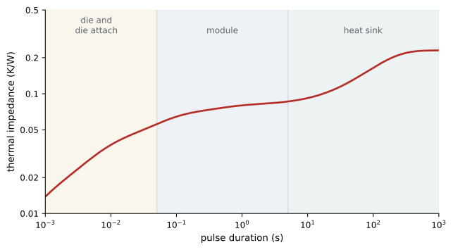
Each layer also stores heat, giving it a thermal capacitance. The combination of resistances and capacitances means that temperatures respond to a change in power with delays: the die heats within milliseconds, the baseplate within seconds, and a large heat sink over minutes. Data sheets describe this with a transient thermal impedance curve, \(Z_{th}(t)\), the temperature rise after a step of 1 W applied for time \(t\), usually fitted by a Foster network of parallel resistance-capacitance pairs:

where \(R_i\) and \(\tau_i\) are the resistance and time constant of each term. For a short pulse, only the fast terms have time to respond, so the junction can absorb large short overloads without exceeding its limit; for long loads, all terms respond and the steady-state resistance applies.

import numpy as np

# Transient thermal impedance of an IGBT module (Foster network) plus heat sink
R = np.array([0.010, 0.025, 0.030, 0.015, 0.150])     # K/W: four junction-to-case terms, then heat sink
tau = np.array([0.0005, 0.005, 0.05, 0.4, 120.0])     # time constants, s

def Z(t):
    return np.sum(R * (1 - np.exp(-t / tau)))

for t in (0.001, 0.01, 0.1, 1, 10, 100, 1000):
    print(f"t = {t:7.3f} s: Zth = {Z(t):.4f} K/W")
print(f"steady state: {R.sum():.3f} K/W")

# A 10 s overload at 150% current (losses 2.25x of 300 W) starting from steady state at 300 W
Ta, P0 = 40.0, 300.0
P1 = 2.25 * P0
Tj0 = Ta + P0 * R.sum()
for t in (0.1, 1, 10):
    Tj = Tj0 + (P1 - P0) * Z(t)
    print(f"after {t:4.1f} s of overload: Tj = {Tj:5.1f} C")
print(f"if the overload continued indefinitely: Tj = {Ta + P1 * R.sum():.0f} C")

t =   0.001 s: Zth = 0.0138 K/W
t =   0.010 s: Zth = 0.0374 K/W
t =   0.100 s: Zth = 0.0644 K/W
t =   1.000 s: Zth = 0.0800 K/W
t =  10.000 s: Zth = 0.0920 K/W
t = 100.000 s: Zth = 0.1648 K/W
t = 1000.000 s: Zth = 0.2300 K/W
steady state: 0.230 K/W
after  0.1 s of overload: Tj = 133.1 C
after  1.0 s of overload: Tj = 139.0 C
after 10.0 s of overload: Tj = 143.5 C
if the overload continued indefinitely: Tj = 195 C

The output shows that the module's own thermal impedance reaches its steady value of 0.08 K/W within about a second, while the heat sink takes minutes. A 10-second overload at 150 percent current, which multiplies conduction losses by roughly 2.25, raises the junction from about 109 °C to 143.5 °C, within a 150 °C limit; the same overload sustained would drive it to 195 °C and destroy the device. This is why drives can be rated for short overloads, such as 150 percent for 60 seconds every 10 minutes, well beyond their continuous rating, and why their protection uses a thermal model of the devices rather than a simple current limit.

Cooling methods

Cooling is chosen according to the heat flux, the space available and the environment:

• Natural convection: finned heat sinks with no fan, used for low power and where reliability or silence matters; typical sink-to-air resistances are of the order of 1 K/W for a hand-sized extrusion.
• Forced air: fans blowing through finned heat sinks reduce thermal resistance several times, at the cost of fan noise, power, filters and a component (the fan) that wears out. Altitude matters: at 3,000 m, air density is about 30 percent lower than at sea level and cooling capacity falls accordingly, so equipment is derated.
• Liquid cooling: cold plates carrying water-glycol mixtures remove heat fluxes far beyond air, and are standard in traction inverters for electric vehicles and trains, wind turbine converters and high-power drives. Pin-fin baseplates in direct contact with coolant remove the thermal interface layer altogether.
• Two-phase cooling: heat pipes and vapour chambers spread heat with very low resistance using evaporation and condensation inside sealed copper tubes.

Whatever the method, thermal design also includes the enclosure: air must enter cool and leave without recirculating, dust must be filtered or excluded, and the temperature of other components such as capacitors, which tolerate less heat than semiconductors, must be checked.

How power modules wear out

Power modules are built from layers with different coefficients of thermal expansion: silicon expands about 3 parts per million per kelvin, copper about 17 and aluminium about 23. Each time the module heats and cools, the layers try to expand by different amounts, and the joints between them are strained. Over thousands to millions of cycles, this cyclic strain causes fatigue:

• Bond wire lift-off: aluminium wires ultrasonically bonded to the top of the die crack at their heel or detach from the die metallization. Resistance rises, current crowds into the remaining wires, and eventually the device fails.
• Solder fatigue: cracks grow in the solder between the die and substrate, or between substrate and baseplate, increasing thermal resistance; temperatures rise, which accelerates the cracking.
• Metallization reconstruction: the aluminium layer on top of the die roughens, raising resistance.

Two kinds of temperature cycling matter. Power cycling, caused by load changes, creates fast swings in junction temperature over seconds, which mostly stress bond wires and die-attach solder. Thermal cycling, caused by ambient changes and start-stop operation over minutes or hours, stresses the larger solder layers between substrate and baseplate. Applications with frequent load changes, such as elevators, cranes, traction and wind turbines, are dominated by these wear-out mechanisms.

Manufacturers have developed module technologies that last much longer: silver sintering instead of solder for die attach, copper wires or copper clips instead of aluminium bond wires, silicon nitride substrates, and baseplate-free designs. Silicon carbide dies are stiffer than silicon, which changes how stress is distributed, and their higher operating temperatures make advanced packaging particularly important.

Lifetime models

Lifetime under power cycling is commonly modelled by extensions of the Coffin-Manson law, in which the number of cycles to failure falls steeply with the temperature swing \(\Delta T_j\) and also depends on the mean temperature. A widely used form, derived from the German LESIT research project of the 1990s, is:

where \(\alpha\) is about \(-5\), \(E_a\) an activation energy, \(R\) the gas constant and \(T_m\) the mean junction temperature in kelvin. The strong dependence on \(\Delta T_j\) means that halving the temperature swing can extend life by a factor of about 30.

Electrolytic capacitors wear out by a different mechanism: the liquid electrolyte slowly evaporates through the seal, reducing capacitance and raising equivalent series resistance (ESR), which further heats the capacitor. Their life roughly doubles for every 10 °C reduction in core temperature, an Arrhenius relationship, so manufacturers rate them at a maximum temperature (often 105 °C) for a certain number of hours and designers calculate life at the actual operating temperature, including the self-heating from ripple current.

import math

# Power-cycling lifetime of bond wires and solder (LESIT-type model, illustrative parameters)
def cycles_to_failure(dT, Tm_C):
    Tm = Tm_C + 273.15
    return 640 * dT ** -5 * math.exp(78000 / (8.314 * Tm))

per_day = 300                                    # load cycles per day (an elevator drive)
for dT, Tm in ((60, 90), (50, 85), (40, 80), (30, 75)):
    N = cycles_to_failure(dT, Tm)
    print(f"swing {dT} K, mean {Tm} C: {N:10.3g} cycles, {N / per_day / 365:7.1f} years at {per_day} cycles/day")

# Electrolytic capacitor life roughly doubles for every 10 C reduction
L0, T0 = 5000.0, 105.0                           # rated hours at rated temperature
for T in (95, 85, 75, 65):
    L = L0 * 2 ** ((T0 - T) / 10)
    print(f"capacitor at {T} C: {L:8.0f} h = {L / 8760:4.1f} years of continuous operation")

swing 60 K, mean 90 C:   1.37e+05 cycles,     1.2 years at 300 cycles/day
swing 50 K, mean 85 C:   4.87e+05 cycles,     4.4 years at 300 cycles/day
swing 40 K, mean 80 C:   2.15e+06 cycles,    19.7 years at 300 cycles/day
swing 30 K, mean 75 C:   1.33e+07 cycles,   121.4 years at 300 cycles/day
capacitor at 95 C:    10000 h =  1.1 years of continuous operation
capacitor at 85 C:    20000 h =  2.3 years of continuous operation
capacitor at 75 C:    40000 h =  4.6 years of continuous operation
capacitor at 65 C:    80000 h =  9.1 years of continuous operation

The results illustrate why thermal design is reliability design. A module cycling through 60 K swings 300 times a day might last little more than a year, while one with 40 K swings would last about 20 years. Capacitors rated 5,000 hours at 105 °C last only about a year at 95 °C but about nine years at 65 °C. Designers therefore size heat sinks and choose devices not only to stay below maximum temperatures, but to keep temperature swings and capacitor temperatures low, and they calculate life from a realistic mission profile: the sequence of loads and ambient temperatures the equipment will see over its life.

Reliability measures

Reliability engineering describes the probability that equipment works for a specified time under stated conditions. During the useful life of a population of components, after early failures and before wear-out, failures occur at a roughly constant rate \(\lambda\), giving the reliability function and mean time between failures (MTBF):

Failure rates are often expressed in FIT (failures in time), the number of failures per \(10^9\) device-hours. For a system in which every component must work (a series system), failure rates add, so a converter with 400 components each at 20 FIT and a power module at 500 FIT has a total of 8,500 FIT, an MTBF of about 118,000 hours (13 years). An MTBF of 13 years does not mean a unit will last 13 years: with a constant failure rate, only about 37 percent of units survive to the MTBF, and about 7 percent fail in the first year.

Handbook failure rates, from sources such as the older US MIL-HDBK-217 and the European FIDES guide, give rough estimates, but they cannot capture wear-out, which is better predicted by physics-of-failure models like those above. The plot of failure rate over time for a population is often drawn as a bathtub curve: a falling rate of early failures caused by manufacturing defects, a flat region of random failures, and a rising rate as wear-out begins. Manufacturers reduce early failures by screening and burn-in, and designers push wear-out beyond the intended life with thermal margins.

Redundancy improves system availability where downtime is costly. Data centre UPS systems use parallel modules in N+1 arrangements, so that the failure of one module does not drop the load, and hot-swappable modules can be replaced without shutdown. Condition monitoring estimates the remaining life of modules and capacitors in service, for example by tracking the forward voltage of a device at a known current (which rises as bond wires degrade) or the capacitor's ESR, so that maintenance can be planned before failure.