High-power converters: HVDC and FACTS

The largest power electronic converters in the world are found not in factories or vehicles but in the transmission grid. High-voltage direct current (HVDC) links carry thousands of megawatts over hundreds or thousands of kilometres, under the sea and between grids that are not synchronized with each other. Flexible AC transmission systems (FACTS) use similar converters to control voltage and power flow on AC lines, letting existing lines carry more power safely. Canada has been a pioneer in both: the first HVDC scheme to use thyristor valves throughout entered service in New Brunswick in 1972, and Manitoba and Quebec deliver much of their hydroelectric power over HVDC. This lesson explains why direct current is used for transmission, the two converter technologies (line-commutated and voltage-source), the modular multilevel converter, HVDC system configurations, and the main FACTS devices.

Why direct current?

Alternating current won the "war of the currents" in the 1890s because transformers make it easy to change AC voltage, and high voltage is needed to transmit power efficiently. But AC transmission has limits that DC does not share:

• Reactive power. AC lines and especially cables have inductance and capacitance that must be charged every half-cycle. In long overhead lines this limits power transfer and requires series and shunt compensation; in cables the charging current is so large that AC cables longer than about 50 to 100 km carry little useful power. DC cables have no such limit, which is why almost all long submarine and underground links, and connections to distant offshore wind farms, use DC.
• Stability. Power transfer over an AC line depends on the angle between the voltages at its ends and becomes unstable as the angle grows, which limits long lines. A DC link's power is set by its converters, regardless of the angle.
• Asynchronous connection. DC can connect grids that run at different frequencies or are not synchronized, such as Quebec's grid and its neighbours in the Eastern Interconnection, or the 50 Hz and 60 Hz grids in Japan. Back-to-back converter stations, with no line between them, are used for this.
• Line cost and losses. A DC line needs two conductors (or one with a ground or metallic return) instead of three, uses narrower rights-of-way and towers, and has no skin effect or reactive current, so it costs less and loses less per kilometre.

Against these advantages stand the converter stations at each end, which are expensive and have their own losses. HVDC therefore becomes economical beyond a break-even distance, commonly quoted as roughly 600 to 800 km for overhead lines and 50 to 100 km for cables, and wherever asynchronous connection or precise control of power flow is needed.

# Comparing overhead AC and HVDC transmission for 2,000 MW (illustrative costs)
P = 2000.0                                   # MW
hours, price, years, rate = 8760 * 0.7, 60.0, 40, 0.06   # load hours per year, $/MWh, life, discount rate
pv = (1 - (1 + rate) ** -years) / rate       # present value factor for annual costs

def ac(km):
    capital = 150e6 + 2.1e6 * km             # substations plus two 500 kV circuits, compensation every 300 km
    loss_mw = 0.042 * P * km / 1000          # about 4.2% per 1,000 km at this loading
    return capital, loss_mw

def dc(km):
    capital = 700e6 + 1.3e6 * km             # two converter stations plus a +/-500 kV bipole line
    loss_mw = 0.015 * P + 0.030 * P * km / 1000   # 0.75% per station plus about 3% per 1,000 km
    return capital, loss_mw

print("  km    AC total ($M)  DC total ($M)  AC losses (MW)  DC losses (MW)")
for km in (200, 400, 600, 800, 1000, 1500):
    rows = []
    for f in (ac, dc):
        cap, loss = f(km)
        total = cap + loss * hours * price * pv
        rows.append((total / 1e6, loss))
    print(f"{km:5d}  {rows[0][0]:13,.0f}  {rows[1][0]:13,.0f}  {rows[0][1]:14.0f}  {rows[1][1]:14.0f}")

  km    AC total ($M)  DC total ($M)  AC losses (MW)  DC losses (MW)
  200            663          1,193              17              42
  400          1,176          1,519              34              54
  600          1,689          1,845              50              66
  800          2,202          2,172              67              78
 1000          2,715          2,498              84              90
 1500          3,998          3,314             126             120

With these assumptions the two options cost about the same at around 750 km, and HVDC is clearly cheaper at 1,000 km and beyond. The converter stations' losses make DC lossier for short links; the lower line losses per kilometre make it less lossy for long ones. Real comparisons use project-specific costs, which vary widely, and include factors such as the right-of-way available, reliability, and the value of controllability.

Line-commutated converters

Classic HVDC uses line-commutated converters (LCC) built from thyristors. Each converter is a six-pulse or, more commonly, twelve-pulse bridge (two six-pulse bridges fed from transformers with a 30-degree phase difference, as in Lesson 3). Each valve consists of hundreds of thyristors in series, since a single thyristor blocks only about 8 kV. The thyristors are turned on by gate pulses but turn off only when the AC system reverses the current through them, so the converter depends on a sufficiently strong AC network for commutation. The DC voltage is controlled by the firing angle: at angles below 90 degrees the bridge rectifies, and above 90 degrees it inverts, so the same station can act as either rectifier or inverter.

LCC systems have several characteristic features. They consume reactive power, about 50 to 60 percent of their active power, which must be supplied by capacitor banks and filters at each station. They generate characteristic current harmonics of order \(12k \pm 1\) that are removed by large AC filters. They reverse power flow by reversing the DC voltage, while the current keeps its direction, which suits overhead lines and mass-impregnated cables but not the extruded polymer cables used in many modern links. And they can suffer commutation failure if the AC voltage at the inverter dips. In return, LCC offers the highest power ratings (up to about 12 GW at ±1,100 kV on recent links in China), low losses (about 0.7 percent per station) and long experience.

Voltage-source converters

Voltage-source converters (VSC) use devices that can be turned off on command, typically IGBTs, to synthesize an AC voltage of any magnitude and phase from the DC link, as the inverters of Lesson 7 do on a much larger scale. Because they do not rely on the AC system for commutation, VSC stations can control active and reactive power independently, supply weak networks and islands, restart a dead grid (black start), and connect offshore wind farms, which have no strong AC system of their own. Power reverses by reversing the current while the DC voltage keeps its polarity, which allows the use of cross-linked polyethylene (XLPE) cables. VSC stations need much smaller filters, so they take up far less space, which matters on offshore platforms.

Early VSC schemes, from 1997, used two-level and three-level converters switching at high frequency, with losses of 2 to 3 percent per station. Since the first scheme entered service in 2010, nearly all new VSC projects have used the modular multilevel converter, which cut losses to about 1 percent per station and made VSC competitive with LCC for most applications below the very highest power levels.

The modular multilevel converter

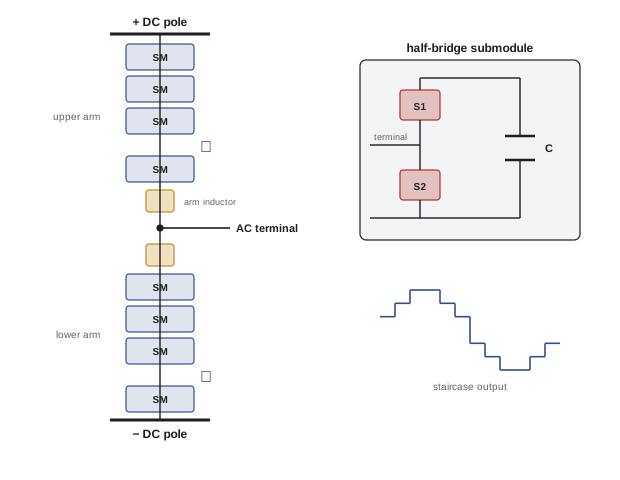
The modular multilevel converter (MMC), invented at the Bundeswehr University Munich around 2001, builds each phase from two arms, each a series string of hundreds of identical submodules plus an arm inductor. In the simplest form, each submodule is a half-bridge with its own capacitor charged to a voltage of about 1.6 to 2.5 kV. Each submodule can either insert its capacitor into the arm or bypass it. By inserting the right number of submodules in the upper and lower arms at each instant, the converter produces a staircase approximation of a sine wave at the AC terminal with as many steps as there are submodules.

import numpy as np

# Modular multilevel converter: waveform quality versus number of submodules, and submodule sizing
def thd_staircase(levels, M=4096):
    t = np.arange(M) / M
    ref = np.sin(2 * np.pi * t)
    v = np.round(ref * (levels - 1) / 2) / ((levels - 1) / 2)    # nearest-level modulation
    spec = np.abs(np.fft.rfft(v))
    return np.sqrt(np.sum(spec[2:200] ** 2)) / spec[1]

for n in (4, 10, 20, 50, 200):
    print(f"{n:3d} submodules per arm ({n + 1} levels): THD {thd_staircase(n + 1):6.2%}")

Vdc, Vsm, redundancy = 640e3, 1.6e3, 1.08        # +/-320 kV link, average submodule voltage
S = 1000e6                                        # VA converter rating
n_arm = int(np.ceil(Vdc / Vsm * redundancy))
E_total = 35e3 * S / 1e6                          # about 35 kJ of stored energy per MVA
E_sm = E_total / (6 * n_arm)
C_sm = 2 * E_sm / Vsm ** 2
print(f"submodules per arm {n_arm} (6 arms, {6 * n_arm} in total)")
print(f"stored energy {E_total / 1e6:.0f} MJ, {E_sm / 1e3:.1f} kJ per submodule, capacitance {C_sm * 1e3:.1f} mF each")

  4 submodules per arm (5 levels): THD 17.32%
 10 submodules per arm (11 levels): THD  7.32%
 20 submodules per arm (21 levels): THD  3.64%
 50 submodules per arm (51 levels): THD  1.33%
200 submodules per arm (201 levels): THD  0.15%
submodules per arm 432 (6 arms, 2592 in total)
stored energy 35 MJ, 13.5 kJ per submodule, capacitance 10.5 mF each

With hundreds of submodules per arm, the staircase is so fine that harmonic distortion is a fraction of a percent, and little or no filtering is needed. Each submodule switches only rarely, at an average of perhaps 100 to 200 Hz, so switching losses are low. A ±320 kV converter needs over 400 submodules per arm, more than 2,500 in all, including redundant submodules that allow the converter to keep operating if some fail (a failed submodule is bypassed by a fast switch). The capacitors store tens of megajoules in total and make up a large part of the converter's volume and cost.

The control of an MMC is demanding. It must keep the thousands of capacitor voltages balanced, typically by sorting the submodules by voltage and choosing which to insert according to the direction of the arm current; control the circulating current that flows between the arms; and protect against DC faults. Half-bridge submodules cannot block current from the AC side into a DC short circuit, so DC faults on overhead lines are cleared by opening AC breakers, or by using full-bridge submodules, which can produce negative voltage and block fault current, at the cost of more semiconductors and higher losses.

HVDC configurations and Canadian examples

HVDC schemes take several forms:

• Monopole: one high-voltage conductor with a return through the ground, sea or a metallic conductor.
• Bipole: two conductors at opposite polarities, the most common configuration for overhead lines; if one pole fails, the other can continue at half capacity.
• Back-to-back: rectifier and inverter in the same station, used to connect asynchronous grids.
• Multi-terminal: three or more stations on one DC network, made easier by VSC technology, and the basis of proposed offshore grids linking many wind farms.

Canada's HVDC links illustrate each type. The Eel River back-to-back station, connecting New Brunswick and Quebec, was the first HVDC scheme to use thyristor valves throughout when it entered service in 1972. Manitoba Hydro's Nelson River system brings power from northern generating stations to southern Manitoba over three bipoles, the newest of which, Bipole III, entered service in 2018 at ±500 kV. Hydro-Québec's Quebec–New England link (Phase II) was one of the first multi-terminal HVDC systems, and Hydro-Québec also operates several back-to-back stations connecting its asynchronous grid to neighbouring systems. In Atlantic Canada, the Labrador-Island Link (LCC) carries power from Muskrat Falls to Newfoundland, and the Maritime Link, an early VSC scheme in North America, connects Newfoundland to Nova Scotia by submarine cable.

Flexible AC transmission systems

FACTS devices use power electronics to control the voltage, impedance or phase angle of AC transmission, increasing the power existing lines can carry and improving stability:

• Static VAR compensators (SVC) use thyristor-controlled reactors and thyristor-switched capacitors to supply or absorb reactive power rapidly, holding voltage steady during disturbances. They are a mature technology, used extensively on long transmission systems such as Hydro-Québec's.
• Static synchronous compensators (STATCOM) use voltage-source converters to inject reactive current directly. Unlike an SVC, whose output falls with the square of voltage, a STATCOM can deliver its full current even at low voltage, giving better support during faults, and it is smaller. Modular multilevel designs are now standard.
• Series compensation inserts capacitors in series with long lines to cancel part of their inductance, increasing power transfer. Thyristor-controlled series capacitors (TCSC) make the compensation adjustable and can damp oscillations and avoid subsynchronous resonance with generator shafts.
• The unified power flow controller (UPFC) combines a shunt and a series converter sharing a DC link, controlling voltage, impedance and angle together, though few have been built because of their cost.

As synchronous generators retire, FACTS devices, battery storage and grid-forming inverters increasingly provide the voltage support and system strength that those generators used to supply, a topic developed in ELE-490.