
ELE-203 · Lesson 12 of 12 · 27 min
Two-port networks, circuit simulation and a design project
Many circuits are used as building blocks with an input and an output: amplifiers, filters, transformers, transmission lines, cables. Describing such a block by the relationship between the voltages and currents at its two ports, without looking inside, lets engineers connect blocks, compare them and specify them. This final lesson introduces two-port parameters and the cascade (ABCD) matrix, explains how circuit simulators such as SPICE solve circuits, and finishes with a design project that uses the methods of the whole course to design and verify a filter.
Two-port networks
A two-port has an input port (voltage \(V_1\), current \(I_1\) flowing in) and an output port (\(V_2\), \(I_2\)). For a linear network without internal independent sources, two of the four quantities can be expressed in terms of the other two. The choice gives different parameter sets, each suited to particular uses:
| Parameters | Equations | Typical use |
|---|---|---|
| Impedance (z) | \(V_1 = z_{11}I_1 + z_{12}I_2\); \(V_2 = z_{21}I_1 + z_{22}I_2\) | Networks in series; T-models |
| Admittance (y) | \(I_1 = y_{11}V_1 + y_{12}V_2\); \(I_2 = y_{21}V_1 + y_{22}V_2\) | Networks in parallel; transistor models at high frequency |
| Hybrid (h) | \(V_1 = h_{11}I_1 + h_{12}V_2\); \(I_2 = h_{21}I_1 + h_{22}V_2\) | Bipolar transistor small-signal models |
| Transmission (ABCD) | \(V_1 = AV_2 + BI_2\); \(I_1 = CV_2 + DI_2\) | Cascaded sections; power lines; filters |
Each parameter is measured by setting one port to an open or short circuit. For example, \(z_{11} = V_1/I_1\) with port 2 open (\(I_2 = 0\)), and \(y_{21} = I_2/V_1\) with port 2 shorted (\(V_2 = 0\)). A network is reciprocal (as all networks of R, L, C and transformers are) if \(z_{12} = z_{21}\), equivalently \(AD - BC = 1\).
Worked problem
z-parameters of a T network
A T network has series arms \(Z_a = 10\) Ω and \(Z_b = 20\) Ω and a shunt arm \(Z_c = -j40\) Ω. Find its z-parameters.
Show solution
- Port 2 open: \(V_1 = (Z_a + Z_c)I_1\), so \(z_{11} = 10 - j40\) Ω; \(V_2 = Z_c I_1\), so \(z_{21} = -j40\) Ω.
- Port 1 open: \(z_{22} = Z_b + Z_c = 20 - j40\) Ω and \(z_{12} = Z_c = -j40\) Ω.
Answer: \(z_{11} = 10 - j40\), \(z_{12} = z_{21} = -j40\), \(z_{22} = 20 - j40\) Ω. The equal off-diagonal terms confirm reciprocity.
The cascade (ABCD) matrix
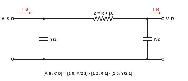
When two-ports are connected in cascade, the output of one feeding the input of the next, their ABCD matrices multiply. This makes ABCD parameters the natural choice for chains of sections: filter ladders, cascaded amplifier stages, and power lines modelled as series impedances and shunt admittances. The two basic elements are
and any ladder is the product of these in order. The input impedance with a load \(Z_L\) on port 2 is \(Z_{in} = (AZ_L + B)/(CZ_L + D)\).
import numpy as np

def series(Z):
    return np.array([[1, Z], [0, 1]], dtype=complex)

def shunt(Y):
    return np.array([[1, 0], [Y, 1]], dtype=complex)

# Nominal-pi model of a 50 km, 138 kV line (per phase): series Z, half the shunt Y at each end
km = 50
Z = (0.10 + 0.50j) * km
Y = 3.3e-6j * km
ABCD = shunt(Y / 2) @ series(Z) @ shunt(Y / 2)
A, B, C, D = ABCD.ravel()
print(f"A = {A:.4f}, B = {B:.2f} ohm, C = {C:.3e} S, D = {D:.4f}")
print(f"reciprocal check AD - BC = {A * D - B * C:.6f}")

# Receiving end: 50 MW at 0.9 pf lagging, 132 kV line-to-line
VR = 132e3 / np.sqrt(3)
IR = 50e6 / (np.sqrt(3) * 132e3 * 0.9) * np.exp(-1j * np.arccos(0.9))
VS, IS = ABCD @ np.array([VR, IR])
print(f"sending voltage {abs(VS) * np.sqrt(3) / 1e3:.1f} kV (line), angle {np.degrees(np.angle(VS)):.2f} deg")
print(f"sending current {abs(IS):.1f} A, receiving current {abs(IR):.1f} A")
PS = 3 * (VS * np.conj(IS)).real
print(f"line loss {(PS - 50e6) / 1e6:.2f} MW, efficiency {100 * 50e6 / PS:.2f}%")
VR_noload = abs(VS) / abs(A)
print(f"voltage regulation {100 * (VR_noload - VR) / VR:.1f}%")A = 0.9979+0.0004j, B = 5.00+25.00j ohm, C = -3.403e-08+1.648e-04j S, D = 0.9979+0.0004j reciprocal check AD - BC = 1.000000+0.000000j sending voltage 138.5 kV (line), angle 3.56 deg sending current 237.3 A, receiving current 243.0 A line loss 0.87 MW, efficiency 98.30% voltage regulation 5.1%
The result shows the reciprocity check \(AD - BC = 1\), a sending voltage of 138.5 kV needed to deliver 132 kV at the load, 0.87 MW of losses, and the line's charging current, which makes the sending current slightly less than the receiving current. The same matrices, with distributed parameters, model long lines in ELE-380.
How circuit simulators work
SPICE (Simulation Program with Integrated Circuit Emphasis), first released at Berkeley in the early 1970s, and its many descendants are used to verify nearly every circuit before it is built. Their core is modified nodal analysis (MNA): nodal analysis extended with an extra unknown, the current, for each voltage source and inductor (in DC), so that any circuit can be written as one matrix equation.
- AC analysis: each element is stamped into a complex matrix at each frequency, which is solved for the node voltages, exactly the phasor method of Lesson 4.
- DC operating point: non-linear devices (diodes, transistors) are linearized and the equations solved iteratively by Newton's method until they converge.
- Transient analysis: capacitors and inductors are replaced at each time step by companion models (a conductance and a current source derived from a numerical integration rule), and the resulting DC problem is solved, step after step, as in the code of Lesson 2.
import numpy as np

# A minimal modified-nodal-analysis (MNA) solver, the core of SPICE-like simulators.
# Netlist: (type, name, node+, node-, value). Node 0 is ground.
netlist = [
    ("V", "Vin", 1, 0, 1.0),        # 1 V AC source
    ("R", "R1", 1, 2, 1000.0),
    ("C", "C1", 2, 0, 31.83e-9),    # third-order Butterworth low-pass, fc = 5 kHz,
    ("L", "L1", 2, 3, 63.66e-3),    # designed for 1 kOhm source and load
    ("C", "C2", 3, 0, 31.83e-9),
    ("R", "RL", 3, 0, 1000.0),
]

def solve(freq):
    s = 2j * np.pi * freq
    n = max(max(e[2], e[3]) for e in netlist)
    vs = [e for e in netlist if e[0] == "V"]
    M = np.zeros((n + len(vs), n + len(vs)), dtype=complex)
    b = np.zeros(n + len(vs), dtype=complex)
    for kind, name, p, q, val in netlist:
        if kind in "RCL":
            y = {"R": 1 / val, "C": s * val, "L": 1 / (s * val)}[kind]
            for i, j, sign in ((p, p, 1), (q, q, 1), (p, q, -1), (q, p, -1)):
                if i and j:
                    M[i - 1, j - 1] += sign * y
    for k, (kind, name, p, q, val) in enumerate(vs):
        row = n + k
        if p:
            M[p - 1, row] += 1; M[row, p - 1] += 1
        if q:
            M[q - 1, row] -= 1; M[row, q - 1] -= 1
        b[row] = val
    return np.linalg.solve(M, b)

for f in (100, 1000, 5000, 10000, 50000):
    x = solve(f)
    v3 = x[2]
    rel = round(20 * np.log10(abs(v3) / 0.5), 1) + 0.0   # relative to the 0.5 (-6 dB) passband level
print(f"f = {f:6d} Hz |V3| = {abs(v3):.4f} relative {rel:6.1f} dB phase {np.degrees(np.angle(v3)):7.1f} deg")f = 100 Hz |V3| = 0.5000 relative 0.0 dB phase -2.3 deg f = 1000 Hz |V3| = 0.5000 relative 0.0 dB phase -23.1 deg f = 5000 Hz |V3| = 0.3536 relative -3.0 dB phase -135.0 deg f = 10000 Hz |V3| = 0.0620 relative -18.1 dB phase 150.3 deg f = 50000 Hz |V3| = 0.0005 relative -60.0 dB phase 101.5 deg
Simulation is only as good as its models. Real components have parasitics: inductors have winding resistance and capacitance between turns, capacitors have series resistance and inductance, and circuit boards add stray inductance and capacitance. Above some frequency, a capacitor behaves like an inductor. Good practice is to simulate with realistic models, sweep component tolerances (Monte Carlo analysis), and confirm with measurement.
Design project: an LC output filter for an inverter
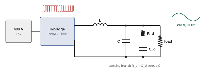
The project brings the course together. A single-phase inverter produces a 60 Hz output by pulse-width modulation (PWM), switching between +400 V and −400 V at 20 kHz. Its output must be filtered so that the load sees a near-sinusoidal 240 V RMS with total harmonic distortion below 3%, at loads up to 5 kW.
Step 1: Choose the corner frequency
An LC low-pass filter attenuates at 40 dB per decade above its resonant frequency \(f_0 = 1/(2\pi\sqrt{LC})\) (Lesson 9). The corner must be well above 60 Hz, so the fundamental passes with little change, and well below 20 kHz, so the switching harmonics are strongly attenuated. A common choice is about one-tenth of the switching frequency: \(f_0 \approx 2\) kHz, giving roughly \(40 \times \log_{10}(20/2) = 40\) dB of attenuation at the switching frequency.
Step 2: Choose L and C
Many pairs give the same \(f_0\). The inductor is sized by the allowed ripple current; the capacitor by the reactive current it draws at 60 Hz. With L = 1 mH:
Worked problem
Component values
With L = 1 mH and \(f_0 = 2\) kHz, find C, its 60 Hz current at 240 V, and the inductor's 60 Hz voltage drop at a full load current of 20.8 A (5 kW at 240 V, resistive).
Show solution
- \(C = 1/((2\pi f_0)^2 L) = 1/((12{,}566)^2 \times 10^{-3}) = 6.3\) µF.
- Capacitor current: \(I_C = 240 \times 2\pi \times 60 \times 6.3 \times 10^{-6} = 0.57\) A, small compared with load current.
- Inductor drop: \(X_L = 2\pi \times 60 \times 10^{-3} = 0.377\) Ω; \(20.8 \times 0.377 = 7.8\) V, at 90° to the output, so the inverter must supply \(\sqrt{240^2 + 7.8^2} = 240.1\) V: negligible.
Answer: C ≈ 6.3 µF (6.8 µF standard). The fundamental is barely affected, as required.
Step 3: Check the switching ripple
The PWM output contains large components near 20 kHz and its multiples. With a 400 V bipolar PWM waveform, the dominant component near the switching frequency can be of the order of 200 V or more. The filter's attenuation at 20 kHz is about \((f_0/f)^2 = (2/20)^2 = 0.01\), so 200 V becomes about 2 V at the output, under 1% of 240 V. Higher harmonics are attenuated more. The output distortion is then dominated by the inverter's own low-order harmonics and the load, and is comfortably under 3%.
Step 4: Damping the resonance
At light load, the LC filter is nearly undamped: its resonance at 2 kHz has a very high Q (Lesson 2), so any excitation near 2 kHz, from the inverter's control or from load changes, produces large ringing. A damping branch of a resistor in series with a capacitor (often a few times C) across the filter capacitor adds damping at resonance without dissipating power at 60 Hz. A resistor of about \(\sqrt{L/C} = \sqrt{10^{-3}/6.8 \times 10^{-6}} = 12\) Ω, the filter's characteristic impedance, gives damping near the optimum.
Step 5: Verify
The design is verified by simulation: an AC sweep shows the transfer function with and without damping; a transient simulation with the actual PWM waveform shows the output voltage and its THD at no load and full load; and a load step from 0 to 5 kW shows the overshoot and settling (Lessons 2 and 10). Component ratings follow from the results: the inductor's peak current (load plus ripple) without saturating, the capacitor's voltage and ripple current, and the damping resistor's power. A prototype is then built and measured, and the measurements compared with the predictions.
Every step used a method from this course: second-order responses and damping, phasors, impedance, power, transfer functions, Bode plots, harmonics, and simulation. That combination of analysis, judgment and verification is what circuit design consists of.
Common mistakes
MistakeMultiplying z-parameter matrices for cascaded networks.
InsteadMultiply ABCD matrices for cascades; add z for series and y for parallel connections.
MistakeForgetting the direction convention for I₂ in ABCD parameters.
InsteadIn ABCD form, I₂ flows out of port 2 toward the load.
MistakeTrusting simulation with ideal component models.
InsteadInclude parasitics and tolerances, and confirm by measurement.
MistakePlacing an LC filter corner close to the switching frequency.
InsteadPlace it about a decade below, and well above the fundamental.
MistakeLeaving an LC filter undamped.
InsteadAdd an RC damping branch near the characteristic impedance √(L/C).
Summary and key terms
- A two-port is described by z, y, h or ABCD parameters, measured with open or short ports.
- Reciprocal networks have z₁₂ = z₂₁, or AD − BC = 1.
- ABCD matrices multiply for cascades; series Z and shunt Y have simple matrices.
- Simulators use modified nodal analysis, Newton iteration and companion models.
- Realistic models, tolerances and measurement are part of verification.
- Filter design combines corner placement, component sizing, damping and simulation.
- Two-port network
- A network characterized by voltages and currents at two ports.
- z-parameters
- Open-circuit impedance parameters.
- y-parameters
- Short-circuit admittance parameters.
- h-parameters
- Hybrid parameters mixing impedance, admittance and gains.
- ABCD parameters
- Transmission parameters relating input to output quantities.
- Reciprocity
- The property that transfer between ports is the same in both directions.
- Nominal-π model
- A line model with series impedance and half the shunt admittance at each end.
- Modified nodal analysis
- Nodal analysis extended with source currents as unknowns.
- Companion model
- A resistive equivalent of a reactive element for one time step.
- Characteristic impedance
- √(L/C), used to size damping for an LC filter.
Practice problems
Work each problem on paper first, then reveal the answer to check.
Which parameter set multiplies for cascaded networks?
Show answer
ABCD.
How is z₁₁ measured?
Show answer
V₁/I₁ with port 2 open.
ABCD of a series 5 Ω impedance?
Show answer
A = 1, B = 5, C = 0, D = 1.
ABCD of series Z followed by shunt Y?
Show answer
[[1 + ZY, Z], [Y, 1]].
Check reciprocity for A = 1.2, B = 10, C = 0.044, D = 1.2.
Show answer
1.44 − 0.44 = 1: reciprocal.
Input impedance of a series 10 Ω two-port loaded with 40 Ω?
Show answer
50 Ω.
What does a simulator do at each transient time step?
Show answer
Replaces L and C with companion models and solves the resulting circuit.
C for f₀ = 1 kHz with L = 2 mH?
Show answer
12.7 µF.
Attenuation of an LC filter one decade above f₀?
Show answer
About 40 dB.
Characteristic impedance for L = 0.5 mH and C = 20 µF?
Show answer
5 Ω.
Lesson quiz · 5 questions
Score 60% or more to complete this lesson.
Create a free account to save your progress, take quizzes and earn a certificate.