
ECON-102 · Lesson 1 of 12 · 29 min
What macroeconomics studies
Macroeconomics is the study of the economy as a whole. Where microeconomics asks how a single household chooses what to buy, or how one firm sets its price, macroeconomics asks why a whole country's output grows faster in some decades than others, why millions of people can lose their jobs at the same time, why the general level of prices sometimes rises quickly and sometimes barely moves, and what governments and central banks can do about it. ECON-101 built the toolkit of supply, demand, costs and market structures. This course uses some of those tools, adds new ones, and applies them to the big numbers that appear in the news every month: gross domestic product, the unemployment rate, inflation, interest rates, exchange rates and government deficits. Finance topics such as valuing bonds and stocks or building a portfolio are covered in FIN-201 and FIN-301; here we focus on how the economy works and how policy affects it.
Macroeconomic questions matter to everyone, not just to economists. Whether a graduate finds a good job quickly depends partly on whether the economy is expanding or in recession. Whether a family can afford a mortgage depends on interest rates set, indirectly, by the central bank. Whether wages keep up with the cost of groceries depends on inflation. And whether a government can fund health care and pensions in twenty years depends on economic growth and on how much debt it accumulates today. Understanding macroeconomics helps you read the news critically, make better personal financial decisions and take part in public debates about policy.
The big questions
Macroeconomists study a handful of central questions. The first is long-run growth: why are some countries rich and others poor, and why do living standards rise over time? Over the past century, real income per person in Canada and the United States has risen roughly sevenfold, a change that dwarfs any recession. The second is short-run fluctuations: why does output sometimes fall and unemployment rise sharply, as in 2008–2009 and in the spring of 2020? The third is the price level: what causes inflation, why did it surge in 2021–2022 after decades of stability, and why did it rise again in parts of 2026 when energy prices jumped? The fourth is the open economy: how do trade, capital flows and exchange rates connect countries? And the fifth is policy: what can monetary policy, run by central banks, and fiscal policy, run by governments through taxes and spending, do to promote growth, stable prices and high employment?
These questions are linked. A policy that boosts spending today may lower unemployment in the short run but raise inflation if the economy is already near capacity. A large government deficit may support demand during a recession but, if it persists for decades, may raise interest rates and crowd out private investment. Much of macroeconomics is about these trade-offs between the short run and the long run, and about the uncertainty that surrounds them.
The business cycle
Real gross domestic product, the inflation-adjusted value of everything an economy produces, does not grow smoothly. It rises in expansions and falls in contractions. The pattern of fluctuations around the long-run trend is called the business cycle, although the word cycle is misleading: expansions and contractions vary greatly in length and depth, and they do not repeat on a regular schedule. A peak is the high point before a downturn; a trough is the low point before recovery. Potential output is the level of output the economy can produce when its resources are fully employed without putting upward pressure on inflation. The output gap is the difference between actual and potential output, expressed as a percentage of potential: a negative gap means slack, and a positive gap means the economy is running hot.
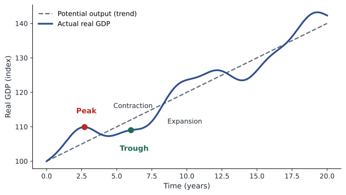
A common rule of thumb defines a recession as two consecutive quarters of falling real GDP. Official judgements are broader.
In Canada, the C.D. Howe Institute's Business Cycle Council, a group of independent economists, dates recessions using the depth, duration and breadth of declines in output and employment. It has identified recessions including 1981–1982, 1990–1992, 2008–2009 and the short, deep pandemic recession of 2020.
Because these committees wait for revised data, they usually announce a peak or trough months after it happens. In the meantime, economists watch leading indicators, such as building permits, new orders, stock prices and the slope of the yield curve, that tend to turn before the economy as a whole.
Worked problem
Growth rates from GDP data
Real GDP (in billions of chained dollars) is 2,300 in year 1, 2,346 in year 2 and 2,334 in year 3. Find the growth rate in each year and describe the change.
Show solution
- Growth rate = (new − old) ÷ old × 100.
- Year 2: (2,346 − 2,300) ÷ 2,300 × 100 = 2.0 %.
- Year 3: (2,334 − 2,346) ÷ 2,346 × 100 = −0.5 %.
Answer: Output grew 2.0 % and then shrank 0.5 %. One year of decline is not necessarily a recession; a dating committee would examine how deep, long and widespread the decline was.
Economists usually report quarterly growth as an annualized rate: the rate at which output would grow over a full year if the quarter's pace continued. A quarter-over-quarter increase of 0.5 % corresponds to an annualized rate of about \( (1.005^4 - 1) \times 100 \approx 2.0 \) %. When you see a headline such as 'the economy grew at a 2 % rate', it is almost always an annualized quarterly figure.
# Growth rates and annualized quarterly growth (illustrative data)
gdp = [2300.0, 2311.5, 2320.8, 2331.2, 2329.0, 2325.1, 2333.4, 2345.0]  # quarterly real GDP
for q in range(1, len(gdp)):
    g = gdp[q] / gdp[q - 1] - 1
    ann = (1 + g) ** 4 - 1
    flag = '  <- decline' if g < 0 else ''
    print(f"Q{q + 1}: quarterly {g * 100:5.2f} %  annualized {ann * 100:5.2f} %{flag}")
yoy = gdp[-1] / gdp[-5] - 1
print(f"Year-over-year growth, last quarter: {yoy * 100:.2f} %")Q2: quarterly 0.50 % annualized 2.02 % Q3: quarterly 0.40 % annualized 1.62 % Q4: quarterly 0.45 % annualized 1.80 % Q5: quarterly -0.09 % annualized -0.38 % <- decline Q6: quarterly -0.17 % annualized -0.67 % <- decline Q7: quarterly 0.36 % annualized 1.44 % Q8: quarterly 0.50 % annualized 2.00 % Year-over-year growth, last quarter: 0.59 %
In this illustrative series, output fell for two consecutive quarters (Q5 and Q6), which would satisfy the rule of thumb for a recession, yet the declines are tiny and output recovers quickly. A dating committee might well decide that this was a pause rather than a recession. The rule of thumb is a useful alarm, not a definition.
Key macroeconomic indicators
Three indicators dominate macroeconomic discussion. Real GDP growth measures how fast output is expanding. The unemployment rate measures the share of people in the labour force who want work but do not have it. The inflation rate measures how fast the general price level is rising, usually using the consumer price index. Alongside these, analysts watch interest rates, the exchange rate, wage growth, productivity, the government budget balance and the current account balance. Each indicator is published by a statistical agency according to international standards, which makes it possible to compare countries and to track changes over time.
| Indicator | Main source in Canada | Release frequency |
|---|---|---|
| Real GDP | Statistics Canada, national accounts | Monthly (by industry) and quarterly (expenditure) |
| Unemployment rate | Statistics Canada, Labour Force Survey | Monthly |
| Consumer price index | Statistics Canada | Monthly |
| Policy interest rate | Bank of Canada | Eight scheduled decisions a year |
| Federal budget balance | Department of Finance; Parliamentary Budget Officer | Annual budget, updates and monthly fiscal monitor |
Macroeconomic data are revised, sometimes substantially, as more complete information arrives. The first estimate of quarterly GDP is based on partial data; later estimates incorporate tax records, business surveys and annual benchmarks. A quarter first reported as weak growth can be revised into a decline, or the reverse. Good analysts treat early figures as provisional and look at several indicators together rather than relying on a single number.
A snapshot of the economy in autumn 2026
To make the indicators concrete, here is the Canadian picture as of mid-October 2026. The unemployment rate was 6.5 % in September, after employment fell by 68,000 that month, with losses concentrated in public services, education and among young workers. Consumer prices were 3.1 % higher than a year earlier, pushed up by energy: gasoline prices were nearly 28 % higher than in September 2025 after a global oil price shock that followed the outbreak of war between the United States and Iran in late February 2026. Excluding gasoline, inflation was 2.2 %, and the Bank of Canada's preferred core measures were close to 2 %. The Bank of Canada had held its policy interest rate at 2.25 % at every decision in 2026, after cutting it from 5 % between June 2024 and October 2025. Real GDP grew about 1.6 % in 2025, and the federal government's spring 2026 economic statement projected growth of about 1.1 % for 2026.
These numbers will be out of date by the time you read this lesson, and that is the point: macroeconomics is a living subject. A useful habit is to check the latest releases yourself. Throughout the course, the portfolio tasks ask you to find current figures from official sources and interpret them with the tools you are learning.
Models and schools of thought
Macroeconomists use models: simplified representations that focus on a few key relationships. The circular flow model in lesson 2 shows how spending, income and production are linked. The aggregate demand and aggregate supply model in lesson 9 explains short-run fluctuations in output and prices. The Solow growth model in lesson 5 explains long-run growth. The loanable funds model in lesson 6 explains interest rates. No model captures everything, and the art of macroeconomics lies in choosing the right model for the question.
Disagreements among macroeconomists are real but often exaggerated. Classical economists emphasized that markets adjust and that, in the long run, output is determined by real resources and technology rather than by money. John Maynard Keynes, writing during the Great Depression of the 1930s, argued that prices and wages adjust slowly, so that economies can remain below potential for long periods unless government spending makes up for weak private demand. Monetarists, led by Milton Friedman, stressed the role of money growth in causing inflation and were sceptical of active fiscal policy. Modern mainstream macroeconomics, sometimes called the new Keynesian synthesis, combines these insights: in the long run output depends on productivity, labour and capital, and inflation depends on monetary policy; in the short run, sticky prices and wages mean that demand matters, and central banks can stabilize the economy by adjusting interest rates. Debates continue about how large fiscal multipliers are, how much debt is too much, and how quickly inflation responds to slack.
| School | Key idea | Policy emphasis |
|---|---|---|
| Classical | Markets clear; money is neutral in the long run | Limited role for stabilization policy |
| Keynesian | Sticky prices; demand can fall short for long periods | Active fiscal policy in downturns |
| Monetarist | Inflation is driven by money growth | Stable, rule-based monetary policy |
| New classical / real business cycle | Fluctuations reflect real shocks and rational responses | Scepticism about fine-tuning |
| New Keynesian | Rational expectations plus sticky prices | Inflation targeting by independent central banks |
Positive and normative macroeconomics
As in ECON-101, it helps to separate positive statements, which describe how the economy works and can in principle be tested, from normative statements, which express values. 'Raising the policy interest rate tends to reduce inflation with a lag of one to two years' is a positive statement. 'The central bank should accept higher unemployment to bring inflation down faster' is a normative one. Many macroeconomic debates mix the two: people may agree on the evidence but weigh unemployment and inflation differently, or care differently about current and future generations when judging government debt. This course aims to give you the positive tools; it is up to you to apply your own values, and to recognize when others are doing the same.
Worked problem
Positive or normative?
Classify each statement: (a) A 1 % fall in the exchange rate raises import prices within a year. (b) The government should run a balanced budget every year. (c) Unemployment rose 0.1 percentage point last month. (d) Inflation is a bigger problem than unemployment.
Show solution
- (a) Positive: a testable claim about cause and effect.
- (b) Normative: a value judgement about what policy should be.
- (c) Positive: a factual statement that can be checked against data.
- (d) Normative: depends on how one weighs the costs of each.
Answer: Statements (a) and (c) are positive; (b) and (d) are normative.
How this course is organized
Lessons 2 to 4 cover measurement: how GDP, inflation and unemployment are defined and calculated, and what the numbers can and cannot tell us. Lessons 5 and 6 cover the long run: economic growth, productivity, saving, investment and the financial system. Lessons 7 and 8 cover money, banking and the central bank. Lessons 9 and 10 bring these together in the short run, using aggregate demand and aggregate supply to analyse recessions, inflation and fiscal policy. Lesson 11 opens the economy to trade, capital flows and exchange rates. Lesson 12 examines the major policy debates and asks you to analyse a real economic briefing.
Common mistakes
MistakeA recession is simply any quarter in which GDP falls.
InsteadRecessions are judged by the depth, duration and breadth of declines in output and employment; two falling quarters is only a rule of thumb.
MistakeMacroeconomics is just microeconomics added up.
InsteadAggregation creates new questions, such as general price inflation and economy-wide unemployment, and new feedbacks between spending and income.
MistakeThe first GDP estimate is the final word.
InsteadGDP is revised several times as fuller data arrive, sometimes changing the picture substantially.
MistakeCapital means money.
InsteadIn economics, capital means produced means of production such as machines, buildings and software.
MistakeEconomists disagree about everything.
InsteadThere is broad agreement on core relationships; debates focus on magnitudes, timing and values.
Summary and key terms
- Macroeconomics studies the economy as a whole: growth, fluctuations, inflation, unemployment, trade and policy.
- Real GDP fluctuates around potential output; the output gap measures slack or overheating.
- Recessions are dated by expert committees using several indicators, not just two quarters of decline.
- Quarterly growth is usually reported at an annualized rate.
- Key data come from national statistical agencies and are revised over time.
- Macroeconomic models simplify; modern mainstream thinking combines Keynesian short-run and classical long-run insights.
- Separating positive from normative statements clarifies policy debates.
- Macroeconomics
- The study of the economy as a whole.
- Real GDP
- The value of final output measured in constant prices.
- Business cycle
- Fluctuations of output and employment around their long-run trend.
- Potential output
- The output an economy can produce with full employment of resources without rising inflation.
- Output gap
- The percentage difference between actual and potential output.
- Recession
- A significant, widespread and lasting decline in economic activity.
- Annualized rate
- A quarterly or monthly change expressed as if it continued for a full year.
- Leading indicator
- A series that tends to turn before the overall economy.
- Monetary policy
- Central bank actions on interest rates and money to influence the economy.
- Fiscal policy
- Government decisions about taxes and spending.
Practice problems
Work each problem on paper first, then reveal the answer to check.
Name the five central questions of macroeconomics.
Show answer
Long-run growth, short-run fluctuations, the price level, the open economy and policy.
Define the output gap.
Show answer
Actual output minus potential output, as a percentage of potential.
Real GDP rises from 500 to 512. What is the growth rate?
Show answer
2.4 %.
A quarter grows 0.8 %. What is the annualized rate?
Show answer
About 3.2 % (1.008 to the fourth power minus 1 is 3.24 %).
Why might two quarters of decline not be called a recession?
Show answer
The decline may be too small, short or narrow; employment may keep growing.
Give two leading indicators.
Show answer
Building permits, new orders, stock prices or the yield curve.
Why are GDP data revised?
Show answer
Early estimates rely on partial data that are later replaced by more complete sources.
What did Keynes emphasize?
Show answer
Sticky prices and the possibility that weak demand keeps output below potential for long periods.
Classify: "The central bank should target 3 % inflation."
Show answer
Normative.
Portfolio task: find the latest monthly unemployment rate, CPI inflation rate and policy interest rate for your country and write three sentences describing the state of the economy.
Show answer
Answers vary; should cite official sources and dates.
Lesson quiz · 5 questions
Score 60% or more to complete this lesson.
Create a free account to save your progress, take quizzes and earn a certificate.