Comparing the economics of power options

Data centre owners must compare power options that differ in almost every respect: a utility tariff with monthly bills, an on-site gas plant with large capital costs and fuel risk, a virtual PPA that is a financial hedge rather than physical supply, a nuclear contract starting years from now, and batteries that earn value in several ways at once. Comparing them fairly requires converting costs to common terms, accounting for time and risk, and valuing what really matters to the business, which is often speed to power rather than cost per megawatt-hour. This lesson develops the levelized cost of energy and its limits, total delivered cost, the economics of redundancy and bridging power, net present value analysis with uncertainty, and the valuation of time to power.

Levelized cost of energy

The levelized cost of energy (LCOE) is the constant price per MWh that would recover a resource's lifetime costs, including a return on capital. For a plant with capital cost \(C\) per kW, fixed operating costs \(F\) per kW-year, variable costs (fuel and variable maintenance) \(V\) per MWh, and capacity factor CF:

where the capital recovery factor (CRF) converts the capital cost into an equal annual payment over \(n\) years at discount rate \(r\), and \(8.76 \cdot \mathrm{CF}\) is the MWh produced per kW per year.

import numpy as np

def crf(r, n):                                          # capital recovery factor
    return r * (1 + r) ** n / ((1 + r) ** n - 1)

def lcoe(capex_kw, fixed_kw_yr, var_mwh, heat_rate, gas, cf, life, r=0.08):
    annual_mwh_per_kw = 8.76 * cf                       # MWh per kW-year
    capital = capex_kw * crf(r, life) / annual_mwh_per_kw
    fixed = fixed_kw_yr / annual_mwh_per_kw
    fuel = heat_rate * gas
    return capital, fixed, var_mwh + fuel

options = {
    "combined cycle (on site)": dict(capex_kw=2200, fixed_kw_yr=30, var_mwh=3.0, heat_rate=6.6, gas=3.5, cf=0.90, life=25),
    "reciprocating engines": dict(capex_kw=1800, fixed_kw_yr=25, var_mwh=8.0, heat_rate=8.3, gas=3.5, cf=0.90, life=20),
    "simple-cycle aeroderivatives": dict(capex_kw=1600, fixed_kw_yr=20, var_mwh=6.0, heat_rate=9.3, gas=3.5, cf=0.90, life=20),
    "solid oxide fuel cells": dict(capex_kw=3500, fixed_kw_yr=60, var_mwh=10.0, heat_rate=6.5, gas=3.5, cf=0.90, life=15),
}
for name, p in options.items():
    c, f, v = lcoe(**p)
    print(f"{name:30s}: capital ${c:5.1f} + fixed ${f:4.1f} + fuel and variable ${v:5.1f} = ${c + f + v:6.1f}/MWh")
print("for comparison: a large-load utility tariff of about $75/MWh all-in, or a nuclear PPA in the $80 to $100/MWh range")
# Bridging: on-site engines run only until the grid arrives in year 3, then sit as backup
c, f, v = lcoe(**options["reciprocating engines"])
print(f"engines used only 3 of 20 years: capital and fixed costs over 3 years add about ${(c + f) * 20 / 3:.0f}/MWh unless resold or kept as backup")

combined cycle (on site)      : capital $ 26.1 + fixed $ 3.8 + fuel and variable $ 26.1 = $  56.0/MWh
reciprocating engines         : capital $ 23.3 + fixed $ 3.2 + fuel and variable $ 37.1 = $  63.5/MWh
simple-cycle aeroderivatives  : capital $ 20.7 + fixed $ 2.5 + fuel and variable $ 38.6 = $  61.8/MWh
solid oxide fuel cells        : capital $ 51.9 + fixed $ 7.6 + fuel and variable $ 32.8 = $  92.2/MWh
for comparison: a large-load utility tariff of about $75/MWh all-in, or a nuclear PPA in the $80 to $100/MWh range
engines used only 3 of 20 years: capital and fixed costs over 3 years add about $176/MWh unless resold or kept as backup

At high capacity factors, combined-cycle and engine plants produce power in the range of $55 to $65/MWh under these assumptions, broadly competitive with large-load utility tariffs, while fuel cells cost more but may be faster to deploy and easier to permit. These figures are indicative only: capital costs for gas turbines and engines rose sharply in 2024 and 2025 as demand from data centres outstripped manufacturing capacity, and delivery times for large turbines stretched to several years.

LCOE has important limits for data centre decisions:

• It ignores redundancy: a data centre needing 100 MW of reliable supply from on-site generation must install perhaps 120 to 140 MW (N+1 or N+2, DCE-340), raising the capital cost per MWh delivered.
• It ignores timing: LCOE treats a plant producing in two years and a contract starting in seven years identically.
• It ignores risk: fuel price, carbon policy, technology and regulatory risks differ greatly between options.
• It ignores value: power when needed, hourly carbon-free energy, capacity accreditation and flexibility are worth different amounts.
• A short use period destroys the economics: a plant used for only a few years before the grid arrives must recover its capital over those years or be repurposed.

Total delivered cost

For grid supply, the comparison is with the total delivered cost: energy, capacity, transmission and distribution, demand charges, ancillary services, taxes and riders, minimum bills and the cost of collateral (Lessons 1, 2 and 9). For a PPA-based strategy, the delivered cost combines the utility bill with the PPA settlement (positive or negative) and any shaping or firming costs. A fair comparison builds an annual cost model for each strategy, hour by hour where prices and hourly matching matter, over the life of the decision, and converts it to a present value.

Net present value and uncertainty

Decisions that unfold over years are compared by net present value (NPV): the sum of future cash flows discounted at a rate reflecting the cost of capital and risk. Because key inputs are uncertain (energization dates, gas prices, capacity prices, load ramps, technology costs), a single NPV can be misleading. Better practice:

• Sensitivity analysis: change one input at a time to see which matter most.
• Scenario analysis: define consistent futures, such as high gas and carbon prices or fast grid buildout, and evaluate each option in each.
• Monte Carlo simulation: draw inputs from distributions and compute the distribution of NPV, reporting the median, downside percentiles and probability of loss.
• Real options thinking: value the flexibility to wait, expand, switch or abandon, for example holding a site option or a queue position whose value lies in what it allows later.

The value of time to power

For AI campuses in particular, the value of operating capacity is so high that time to power often dominates every other consideration. If a megawatt of operating AI compute generates gross margin of $1 million to $2 million a year, a 200 MW campus energized a year earlier earns $200 to $400 million more, far exceeding plausible differences in energy cost. This is why developers pay premiums for sites with existing connections, accept large-load tariffs, build bridging generation and agree to flexible connections.

import numpy as np

rng = np.random.default_rng(10)
N = 10000
margin = 1.5e6                                         # gross margin per MW-year of operating AI capacity
mw = 200
# Option A: wait for the grid. Energization date uncertain: most likely 4 years, range 3 to 7.
grid_year = rng.triangular(3, 4, 7, N)
# Option B: build 200 MW of on-site engines, ready in 2 years (range 1.5 to 3), extra cost $25/MWh while running before grid
onsite_year = rng.triangular(1.5, 2, 3, N)
extra_cost_per_year = 25 * mw * 8760 * 0.9
capex_extra = 200e6                                     # capital for the bridging plant beyond backup needs (partly recoverable)
r = 0.08
def pv(start, end, amount):                             # present value of a constant annual amount from start to end
    t = np.linspace(0, 1, 50)
    return np.array([np.sum(amount * (b - a) / 50 * (1 + r) ** -(a + (b - a) * t)) if b > a else 0.0 for a, b in zip(start, end)])
gain = pv(onsite_year, grid_year, margin * mw - extra_cost_per_year)
npv = gain - capex_extra
print(f"months gained: median {np.median(grid_year - onsite_year) * 12:.0f}")
print(f"NPV of bridging power: median ${np.median(npv) / 1e6:,.0f}M; 10th percentile ${np.percentile(npv, 10) / 1e6:,.0f}M; probability negative {np.mean(npv < 0):.0%}")

months gained: median 29
NPV of bridging power: median $287M; 10th percentile $88M; probability negative 2%

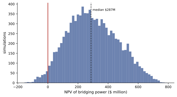
With a median gain of more than two years of operation, bridging power has a median NPV of nearly $300 million and is negative in only about 2% of scenarios, those where the grid arrives early and the bridging plant is late. The analysis also shows the main risk to manage: the bridging plant's own schedule, which depends on equipment delivery, permits and gas supply (Lessons 7 and 8). Reducing that risk, for example by securing equipment early, is worth more than reducing its cost.

Comparing long-term clean supply

Long-term options such as nuclear PPAs, geothermal and long-duration storage (Lessons 6 and 10) are compared on similar principles, with extra attention to:

• Timing: firm clean resources often arrive years after the data centre, so the comparison covers both an interim strategy and the long-term supply.
• Value beyond energy: round-the-clock carbon-free supply has value for hourly matching that LCOE does not capture; its price premium over grid power should be compared with the cost of achieving the same hourly CFE score in other ways (Lesson 6).
• Counterparty and project risk: first-of-a-kind technologies carry construction and cost overrun risk, often shared through contract structures such as fixed-price PPAs with milestone protections, equity stakes or prepayments.
• Policy risk: tax credits, carbon prices and market rules can change materially over a 20-year contract; contracts allocate this risk through change-in-law and price adjustment clauses (Lesson 9).