Energy, sustainability and a cooling design project

Cooling decisions are judged over decades: a plant runs for twenty years or more, and its energy, water and refrigerant use add up to most of its environmental footprint and much of its operating cost. This final lesson shows how annual energy is estimated from climate data, how PUE and water use emerge from design choices, how refrigerants and embodied carbon enter the picture, and how waste heat can become a resource. It ends with a design project that applies the methods of the whole course to the cooling of a 10 MW hall.

Annual energy modelling

Peak conditions size the equipment, but annual energy depends on how the plant runs in every hour of the year. The simplest models use bin hours: the number of hours the outdoor temperature (or wet-bulb temperature, for evaporative systems) falls in each band, from climate data such as ASHRAE design conditions or typical meteorological year (TMY) weather files. For each bin, the model determines the plant's operating mode, free cooling, partial or mechanical, and its power, and sums over the year. Detailed models use hourly simulation, with equipment curves for chillers, towers, pumps and fans and the actual control sequences (Lesson 8).

import numpy as np

# Synthetic hourly dry-bulb temperatures for a cold-continental city (annual and daily cycles)
rng = np.random.default_rng(12)
h = np.arange(8760)
t_out = (4.0 - 14.0 * np.cos(2 * np.pi * (h - 480) / 8760)
         + 5.0 * np.sin(2 * np.pi * (h % 24 - 9) / 24) + rng.normal(0, 3.0, 8760))

it_kw = 10000.0
fwd_supply = 24.0                   # facility water supply setpoint for air handlers, C
approach_dry = 6.0                  # dry cooler approach to outdoor dry-bulb, K

def cooling_power(t):
    # full free cooling, partial, or full mechanical cooling, as kW of cooling-plant power
    free_limit = fwd_supply - approach_dry           # outdoor temperature for full free cooling
    fans_pumps = 0.035 * it_kw                       # always on
    if t <= free_limit:
        return fans_pumps + 0.01 * it_kw, "free"
    frac = min((t - free_limit) / 8.0, 1.0)          # share of load on chillers
    cop = 7.0 - 0.12 * max(t - 20.0, 0.0)            # chiller efficiency falls in hot weather
    return fans_pumps + 0.01 * it_kw + frac * it_kw / cop, "partial" if frac < 1 else "mechanical"

powers, modes = zip(*(cooling_power(t) for t in t_out))
powers = np.array(powers)
other = 0.04 * it_kw                                 # electrical losses, lighting and so on
pue = (it_kw + powers + other) / it_kw
for m in ("free", "partial", "mechanical"):
    print(f"{m:10s} hours: {modes.count(m):5d}")
annual_pue = (it_kw * 8760 + powers.sum() + other * 8760) / (it_kw * 8760)
print(f"annual cooling energy {powers.sum() / 1000:7.0f} MWh; annual PUE {annual_pue:.3f}; worst hour {pue.max():.3f}")

free       hours:  7764
partial    hours:   956
mechanical hours:    40
annual cooling energy    4533 MWh; annual PUE 1.092; worst hour 1.262

With warm facility water and dry coolers, this climate allows free cooling for almost 90% of the year, and the annual PUE is near 1.09. The worst hour, on a hot afternoon, is much higher, which matters for electrical capacity: the electrical system must supply the peak cooling power, while the annual energy depends on the average. Changing a single design choice, the facility water supply temperature, shifts the free-cooling boundary by the same number of degrees and can change annual energy substantially; the model makes such trade-offs visible.

Efficiency metrics

Lesson 1 introduced PUE (total facility energy divided by IT energy). Its main companions are:

• Water usage effectiveness (WUE): litres of site water per kWh of IT energy (Lesson 7). Evaporative systems lower PUE but raise WUE; dry systems do the reverse.
• Carbon usage effectiveness (CUE): kilograms of CO₂-equivalent per kWh of IT energy, depending on PUE and the carbon intensity of the electricity supply.
• Energy reuse effectiveness (ERE) and energy reuse factor (ERF): measures of how much energy is exported as reused heat.

These metrics are defined in the ISO/IEC 30134 series and are increasingly reported to regulators: the European Union's Energy Efficiency Directive requires data centres above 500 kW to report energy, water and heat-reuse data, and some jurisdictions have set efficiency or heat-reuse requirements for new facilities.

Refrigerants and embodied carbon

Refrigerants leak over a system's life, and many have a global warming potential (GWP) thousands of times that of CO₂. Regulations under the Kigali Amendment to the Montreal Protocol, implemented in Canada through federal regulations and in the United States through the AIM Act, are phasing down high-GWP hydrofluorocarbons such as R-410A and R-134a in favour of lower-GWP refrigerants such as R-1234ze, R-513A, R-32 and natural refrigerants (Lesson 5). Designs that minimize refrigerant charge, such as central chillers rather than many DX units, or no compressors at all where climate allows, reduce this risk.

Embodied carbon, the emissions from manufacturing and installing equipment, piping, structure and buildings, is a growing part of the footprint as operational emissions fall with cleaner electricity. Cooling contributes through chillers, dry coolers, pipe and steel. Lifecycle assessment (following ISO 14040 and EN 15978 for buildings) compares options over their whole lives.

Heat reuse

Almost all the electricity a data centre uses becomes heat. Reusing it to heat buildings, greenhouses, pools or industrial processes displaces other fuels. The obstacles are temperature and location:

• Air-cooled data centres reject heat at 25 °C to 35 °C, too cold for most district heating networks, which typically supply 60 °C to 90 °C (newer low-temperature networks run cooler).
• Liquid cooling raises the available temperature to 40 °C to 60 °C, closer to useful.
• Heat pumps can lift the temperature further, using electricity; their efficiency (COP) is highest when the lift is small.
• A heat consumer must be nearby and need heat when the data centre produces it, which in practice means the heating season, unless the heat is stored or used for processes year-round.

# Heat reuse: lifting 35 C data centre water to 70 C for district heating with a heat pump
it_mw = 10.0
recoverable = 0.85 * it_mw            # MW of heat in the liquid loop
t_source, t_supply = 35.0 + 273.15, 70.0 + 273.15
carnot = t_supply / (t_supply - t_source)
cop = 0.5 * carnot                    # real heat pumps reach about half of Carnot
heat_out = recoverable * cop / (cop - 1)      # MW delivered = source heat + compressor work
work = heat_out - recoverable
print(f"Carnot COP {carnot:.1f}, realistic COP {cop:.1f}")
print(f"from {recoverable:.1f} MW of waste heat: {heat_out:.1f} MW to the network, {work:.1f} MW of electricity")

hours = 5000                           # heating-season hours when the network can take the heat
price = 30.0                           # $ per MWh of heat sold
elec = 80.0                            # $ per MWh of electricity
revenue = heat_out * hours * price
cost = work * hours * elec
homes = heat_out * hours / 15.0        # about 15 MWh of heat per home per year
print(f"heat sold {heat_out * hours:,.0f} MWh/yr: revenue ${revenue:,.0f}, electricity ${cost:,.0f}, homes heated about {homes:,.0f}")

Carnot COP 9.8, realistic COP 4.9
from 8.5 MW of waste heat: 10.7 MW to the network, 2.2 MW of electricity
heat sold 53,391 MWh/yr: revenue $1,601,744, electricity $871,316, homes heated about 3,559

Examples include data centres in Nordic countries connected to district heating networks, and projects in Canada and elsewhere that heat greenhouses, university campuses and residential districts. Successful projects are planned with the heat consumer from the start: site selection near heat demand, liquid cooling at the highest feasible temperature, space and power for heat pumps, and contracts that share costs and benefits.

Design project: cooling a 10 MW hall

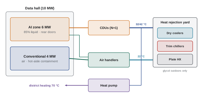
The project combines the course's methods. A developer plans a 10 MW IT hall near Edmonton, Alberta (cold continental climate, ASHRAE 0.4% summer design dry-bulb near 28 °C, winters below −30 °C). The tenant expects a mix: 6 MW of AI racks at 120 kW with 85% liquid cooling, and 4 MW of conventional racks at 15 kW, air cooled. A small district heating network nearby could take some heat.

Step 1: Loads and split

AI zone: 6 MW, of which \(0.85 \times 6 = 5.1\) MW to liquid and 0.9 MW to air. Conventional zone: 4 MW to air. Total air-side load: 4.9 MW; liquid: 5.1 MW (Lessons 1 and 10).

Step 2: Temperatures

Two facility water temperatures suit the two kinds of load: a warm loop for the CDUs, about 32 °C supply and 42 °C return, set by the chips' temperature chain with margin (Lesson 10); and a cooler loop, about 20 °C to 22 °C supply, for air handlers delivering 24 °C to 26 °C supply air within the ASHRAE recommended range with coils that run dry (Lessons 2 and 4).

Step 3: Air side

The conventional zone uses hot-aisle containment and fan walls or CRAHs selected at actual return-air and water temperatures, N+1 (Lessons 3 and 4). The AI zone's 0.9 MW of residual air heat is handled by rear-door heat exchangers on the warm loop where the door can be room-neutral, plus room air handlers. Aisle pressure control sets fan speeds; supply air temperature control sets valves (Lesson 8).

Step 4: Heat rejection and economization

Dry coolers serve both loops, with glycol confined to the outdoor circuit by plate heat exchangers because of the severe winters (Lesson 6). With 32 °C supply, the warm loop can be cooled by dry coolers whenever the outdoor temperature is below about 26 °C, nearly all year. The cool loop gets full free cooling below about 14 °C and partial free cooling above, with trim chillers for the warmest hours (Lessons 5 and 7). Evaporative cooling is avoided to conserve water, accepting a slightly higher peak power; WUE is close to zero.

Step 5: Hydronics and reliability

Each loop has variable-speed pumps (N+1) on UPS, looped headers, ΔT design of 10 K, and pressure-independent valves (Lesson 6). CDUs are N+1 per row group; storage on the cool loop rides through trim chiller restarts. Common-mode risks are checked: separate electrical feeds, separate piping paths, controls on redundant PLCs with UPS (Lesson 11).

Step 6: Annual performance and heat reuse

An hourly model, like the code example, estimates annual PUE near 1.1 and peak cooling power for electrical sizing. A heat pump taking 2 MW to 4 MW from the warm loop in winter serves the district network, and the business case is tested with the network operator (Q14 shows the method).

Step 7: Commission and operate

Integrated systems tests with air and liquid load banks verify capacity, controls, failures and restarts before the tenant arrives; operations then trend ΔT, approach temperatures and economizer hours to keep the plant at its design efficiency (Lessons 8 and 11).

Each step drew on earlier lessons. Cooling design is a chain of decisions, from the chip's temperature limit to the climate outside, and the best designs keep that whole chain in view.