
CHE-350 · Lesson 5 of 12 · 21 min
Rigorous stage-by-stage calculations
Graphical and shortcut methods design a column. Before Ingrid seals the recovery column's design basis, she wants it rated: given the 17 stages, the feed on stage 11 and a reflux ratio of 1.59, what products does the column actually make when the equilibrium is calculated properly on every stage? That is a rigorous calculation. Every process simulator does it, and Theo's goal this week is to understand what the simulator is doing well enough to judge when to trust it. He writes a small version himself.
The MESH equations
A rigorous model writes four kinds of equations for every stage \(j\) and every component \(i\), named by their initials:
| Letter | Equation | Meaning |
|---|---|---|
| M | \(L_{j-1}x_{i,j-1} + V_{j+1}y_{i,j+1} + F_j z_{i,j} - L_j x_{i,j} - V_j y_{i,j} = 0\) | Material balance for each component |
| E | \(y_{i,j} = K_{i,j}\,x_{i,j}\) | Phase equilibrium on each stage |
| S | \(\sum_i x_{i,j} = 1,\ \sum_i y_{i,j} = 1\) | Mole fractions sum to one |
| H | \(L_{j-1}h_{j-1} + V_{j+1}H_{j+1} + F_j h_{F,j} - L_j h_j - V_j H_j + Q_j = 0\) | Energy balance on each stage |
For a column with \(N\) stages and \(c\) components there are about \(N(2c + 3)\) equations, all coupled. The K-values depend on temperature and on composition through the activity coefficients, and the enthalpies depend on both. No closed-form solution exists; the equations are solved iteratively. The methods differ in how they group the equations and in which variables they update first.
The bubble-point method
For distillation of mixtures with a moderate boiling range, the bubble-point method, published by Wang and Henke in 1966, is the classic choice. It uses one key observation: if the temperatures and flows on every stage are fixed, the K-values are fixed, and the material balance for each component becomes a set of linear equations. Substituting \(y = Kx\) into the M equation gives, for each component,
Each stage links only to the stages above and below it, so the equations form a tridiagonal matrix that the Thomas algorithm solves directly, in a single sweep down and back up. The method then normalises the liquid mole fractions on each stage so they add to one, finds each stage's bubble-point temperature from those compositions, updates the K-values, and repeats until the temperatures stop changing. With constant molar overflow, as here, the flows stay fixed; a full version would also update them from the energy balances on each pass.
The program
Theo's program applies the method to the recovery column. The specification is the one a column operator would give: number of stages, feed stage, distillate flow and reflux ratio. The total condenser sits above stage 1, so the reflux entering stage 1 has the composition of the gas leaving it, and stage 17 is the reboiler. The K-values come from the same van Laar model and Antoine equations as before.
# Rating the rectifier stage by stage: a bubble-point (Wang-Henke) method with constant molar overflow
import math
# Ethanol (1) - water (2) at 1 atm: Antoine (mmHg, deg C) and van Laar constants fitted in CHE-320
ANT = {'ethanol': (8.20417, 1642.89, 230.300), 'water': (8.07131, 1730.63, 233.426)}
A12, A21 = 1.672, 0.930
def psat(c, T):  # kPa
    a, b, cc = ANT[c]
    return 10 ** (a - b / (T + cc)) * 0.133322
def gammas(x1):
    x2 = 1 - x1
    d = A12 * x1 + A21 * x2
    return math.exp(A12 * (A21 * x2 / d) ** 2), math.exp(A21 * (A12 * x1 / d) ** 2)
def bubble(x1, P=101.325):
    g1, g2 = gammas(x1)
    lo, hi = -20.0, 250.0
    for _ in range(60):
        T = (lo + hi) / 2
        s = x1 * g1 * psat('ethanol', T) + (1 - x1) * g2 * psat('water', T)
        lo, hi = (T, hi) if s < P else (lo, T)
    y1 = x1 * g1 * psat('ethanol', T) / P
    return T, y1
N, f = 17, 11                 # stage 1 = top tray (total condenser above it), stage 17 = reboiler, feed on stage 11
F, zF, D, R = 100.0, 0.10, 12.45, 1.59
L = [R * D if j < f - 1 else R * D + F for j in range(N)]; L[N - 1] = F - D   # liquid leaving each stage
V = [(R + 1) * D] * N                                                        # gas leaving each stage
Fj = [0.0] * N; Fj[f - 1] = F
P = 101.325
def K(c, x1, T):
    g1, g2 = gammas(x1)
    return (g1 * psat('ethanol', T) if c == 0 else g2 * psat('water', T)) / P
def thomas(a, b, c, d):
    n = len(d); cp, dp = [0.0] * n, [0.0] * n
    cp[0], dp[0] = c[0] / b[0], d[0] / b[0]
    for i in range(1, n):
        m = b[i] - a[i] * cp[i - 1]
        cp[i] = c[i] / m if i < n - 1 else 0.0
        dp[i] = (d[i] - a[i] * dp[i - 1]) / m
    x = [0.0] * n; x[-1] = dp[-1]
    for i in range(n - 2, -1, -1): x[i] = dp[i] - cp[i] * x[i + 1]
    return x
T = [78 + 22 * j / (N - 1) for j in range(N)]
x1 = [0.5 - 0.5 * j / (N - 1) for j in range(N)]
for it in range(400):
    xs = []
    for c, zc in ((0, zF), (1, 1 - zF)):
        Kj = [K(c, x1[j], T[j]) for j in range(N)]
        a = [0.0] + [L[j - 1] for j in range(1, N)]
        # total condenser: distillate D leaves as liquid from stage 1's rising gas; stage 1 receives reflux of composition y1
        b = [-(V[j] * Kj[j] + L[j]) for j in range(N)]
        b[0] = -(V[0] * Kj[0] + L[0]) + R * D * Kj[0]     # reflux returns the top gas composition
        c_ = [V[j + 1] * Kj[j + 1] for j in range(N - 1)] + [0.0]
        d = [-Fj[j] * zc for j in range(N)]
        xs.append(thomas(a, b, c_, d))
    s = [xs[0][j] + xs[1][j] for j in range(N)]
    x1 = [xs[0][j] / s[j] for j in range(N)]
    Tn = [bubble(min(max(x, 1e-9), 0.999))[0] for x in x1]
    err = max(abs(a - b) for a, b in zip(Tn, T)); T = Tn
    if err < 1e-6: break
print(f"after {it + 1} passes the largest change in a stage temperature is {err:.1e} C")
print("stage   T (C)    x ethanol   y ethanol")
for j in range(N):
    y = K(0, x1[j], T[j]) * x1[j]
    if j in (0, 1, 3, 5, 7, 9, 10, 11, 13, 15, 16):
        print(f"{j + 1:4d}   {T[j]:6.2f}    {x1[j]:8.4f}    {y:8.4f}")
y1 = K(0, x1[0], T[0]) * x1[0]
print(f"ethanol balance: in {F * zF:.3f}, out {D * y1 + (F - D) * x1[-1]:.3f} kmol/h")
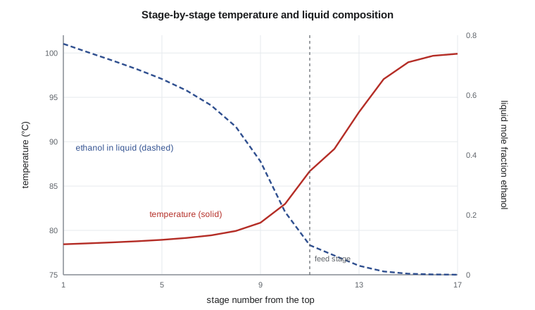
print(f"distillate {y1:.4f} mole fraction ethanol (design 0.80); bottoms {x1[-1]:.5f} (design 0.0005)")after 400 passes the largest change in a stage temperature is 1.4e-04 C stage T (C) x ethanol y ethanol 1 78.44 0.7712 0.8013 2 78.54 0.7431 0.7828 4 78.78 0.6862 0.7485 6 79.15 0.6154 0.7108 8 79.94 0.4943 0.6566 10 82.99 0.2097 0.5418 11 86.67 0.0988 0.4381 12 89.18 0.0642 0.3662 14 97.05 0.0110 0.1107 16 99.68 0.0011 0.0125 17 99.91 0.0003 0.0032 ethanol balance: in 10.000, out 10.000 kmol/h distillate 0.8013 mole fraction ethanol (design 0.80); bottoms 0.00027 (design 0.0005)
Comparing the rigorous answer with McCabe-Thiele
The rigorous calculation predicts a distillate of 80.1 mol % ethanol and bottoms of 0.027 mol %, slightly better than the design targets of 80 % and 0.05 %. The ethanol balance closes to within 0.001 kmol/h. The McCabe-Thiele design was a little conservative, which is expected: stepping off stages graphically rounds the last partial step up to a whole stage, so the staircase's 17 stages actually contained a fraction of a stage spare. Ingrid prefers it that way round. If the rigorous answer had come out worse than the targets, the design would have needed more stages or more reflux.
The temperature profile tells the operators where the column does its work. The top six stages sit within a degree of 78.4 °C, because the liquid there is between 62 and 77 mol % ethanol and the bubble point barely changes with composition. Around the feed the temperature climbs quickly, from 83 °C on stage 10 to 93 °C on stage 13, and the last two stages sit within half a degree of 100 °C.
Using the profile for control
A distillation column is usually controlled through a tray temperature, because composition analysers are slow and expensive. The best tray for control is where the temperature changes most per unit change in product composition, which on this profile is in the steep region a few stages below the feed. A temperature controller on stage 12 or 13, adjusting the reboiler steam, will hold the bottoms specification far better than one on stage 16, where a tenth of a degree corresponds to a large change in ethanol loss. Theo marks stage 13 for the control thermocouple and stages 8 and 10 for indicators, and the profile goes into the operating manual. CHE-374 develops the control design.
Convergence
Theo's program updates the temperatures by direct substitution: compute compositions, compute new bubble points, repeat. It works, but slowly. After 400 passes the largest change in a stage temperature is still about \(10^{-4}\) °C. Direct substitution converges slowly when the K-values change a lot with temperature and composition, as they do here near the feed.
Commercial simulators use faster methods. The sum-rates method, preferred for absorbers and strippers with wide-boiling components, updates the flows from the sums of component flows and the temperatures from the energy balances. Simultaneous-correction methods, such as Naphtali-Sandholm, solve all the MESH equations together by Newton's method and converge in a handful of iterations from a reasonable start. Inside-out methods, the default in most simulators, wrap a fast inner loop on simple approximate K-value and enthalpy models inside an outer loop that updates those models from the rigorous thermodynamics. All of them need a starting guess, which is where the shortcut results of lesson 4 earn their keep.
Worked problem
One tridiagonal row
Write the ethanol balance for stage 10 of the recovery column, in the rectifying section just above the feed, using \(L = 19.79\) and \(V = 32.23\) kmol/h.
Show solution
- Liquid from stage 9 enters: \(19.79\,x_9\).
- Gas from stage 11 enters: \(32.23\,K_{11}x_{11}\).
- Leaving: \(19.79\,x_{10} + 32.23\,K_{10}x_{10}\).
- Row: \(19.79\,x_9 - (32.23K_{10} + 19.79)\,x_{10} + 32.23K_{11}x_{11} = 0\), since stage 10 has no feed.
Answer: Each row has three non-zero terms, so the system is tridiagonal.
What the simulator adds, and what it hides
A commercial simulator would add the energy balances, so the flows vary from stage to stage; a pressure profile, typically 0.5 to 1 kPa per tray; tray efficiencies or a rate-based model; and better thermodynamics, perhaps NRTL with parameters regressed from a large data bank, as discussed in CHE-320. Each addition improves the answer only if the inputs behind it are right. The most common source of error in industrial column simulations is not the solver but the thermodynamic model, and the second is a wrong specification that makes the solver converge to a solution nobody intended.
Ingrid's checklist for any simulator result: check the overall and component balances; check that the temperature profile looks physically sensible, with no stage hotter than the reboiler or colder than the condenser; compare the result with a shortcut or graphical estimate; and change one specification to see if the answer moves in the expected direction. A rigorous model that fails those checks is worse than a back-of-envelope estimate, because it looks authoritative.
Rate-based models
Equilibrium-stage models with efficiencies are standard for trays, but for packed columns, reactive columns and systems where the components transfer at very different rates, rate-based models can be better. They write mass-transfer rate equations between the phases, using the film theory and mass-transfer coefficients of CHE-314, instead of assuming equilibrium. They need hardware details such as packing type and diameter, and more physical properties, and they are slower. For the ethyl acetate line's reactive distillation column, where reaction and mass transfer happen together, the vendor's design was rate-based. Theo's recovery column, with ordinary trays and a well-studied mixture, does not need one.
Common mistakes
MistakeAssuming the simulator's answer is right because it converged.
InsteadCheck balances, profiles and a shortcut estimate before using it.
MistakePutting the control thermocouple near the bottom where the temperature is flat.
InsteadUse a tray where temperature changes most with composition, in the steep part of the profile.
MistakeStarting a rigorous calculation from a poor guess.
InsteadInitialise from shortcut or graphical results.
MistakeBlaming the solver for a wrong answer.
InsteadThe thermodynamic model and the specifications are the usual causes.
Summary and key terms
- Rigorous models solve the MESH equations on every stage.
- The bubble-point method solves tridiagonal component balances, then updates temperatures from bubble points.
- The rated recovery column makes 80.1 mol % distillate and 0.027 mol % bottoms, slightly better than the targets.
- The temperature profile is flat at the top and bottom and steep near the feed; control on a steep tray.
- Simulators use simultaneous-correction or inside-out methods, and must be checked against simpler methods.
- MESH equations
- Material, equilibrium, summation and enthalpy equations for each stage.
- Bubble-point method
- A rigorous method that updates stage temperatures from bubble-point calculations.
- Tridiagonal matrix
- A matrix with non-zero entries only on the diagonal and its two neighbours.
- Thomas algorithm
- A direct solver for tridiagonal systems.
- Inside-out method
- A rigorous method with an inner loop on simple models updated by an outer rigorous loop.
- Rate-based model
- A column model that uses mass-transfer rates instead of equilibrium stages.
Practice problems
Work each problem on paper first, then reveal the answer to check.
How many unknowns are there per stage in a three-component column with variable flows?
Show answer
Three \(x\), three \(y\), \(T\), \(L\) and \(V\): nine.
Why does the bubble-point method use the Thomas algorithm?
Show answer
With fixed K-values and flows, each component's balances form a tridiagonal linear system.
The rigorous bottoms is 0.027 mol % against a target of 0.05 %. Is the design conservative?
Show answer
Yes, slightly; the column does better than specified.
Why is stage 16 a poor control tray?
Show answer
Its temperature barely changes when the ethanol content changes.
Name two checks on any simulator result.
Show answer
Balances close; the temperature profile is physically sensible.
When might a rate-based model be needed?
Show answer
For packed or reactive columns, or when components transfer at very different rates.
Lesson quiz · 5 questions
Score 60% or more to complete this lesson.
Create a free account to save your progress, take quizzes and earn a certificate.