
CHE-350 · Lesson 4 of 12 · 20 min
Multicomponent distillation: shortcut methods
Real feeds rarely contain two components. The ester line's streams carry ester, ethanol, water and acid; the plant's fusel-oil side draws carry four or five alcohols. McCabe-Thiele diagrams cannot represent them, and a full stage-by-stage calculation (lesson 5) needs a starting design. The shortcut methods of this lesson give that starting design in minutes: the minimum number of stages, the minimum reflux, an estimate of the actual stages at a chosen reflux, and the feed location. Simulators still use them to initialise rigorous models, and experienced engineers use them to check simulator answers.
Theo's example comes from a commercial question. Kingfisher Bioenergy and two partner plants each draw off fusel oil, the higher alcohols described in lesson 3. Today they burn it in their boilers. A chemicals buyer has offered a better price for an n-propanol-rich cut, provided the isobutanol content is low. After decanting off the water and drying, the pooled fusel cut is about 2 kmol/h of four alcohols. Ingrid asks whether a small splitter column could make the cut, and roughly how big it would be.
Key components
In a multicomponent separation the designer picks two key components whose split defines the job. The light key is the heaviest component that must mostly go overhead; the heavy key is the lightest component that must mostly go to the bottoms. Components lighter than the light key go almost entirely overhead, and components heavier than the heavy key almost entirely to the bottoms; they are the non-keys. Here the light key is n-propanol and the heavy key isobutanol. Ethanol is a light non-key and isoamyl alcohol a heavy non-key. The specification is 98 % of the n-propanol overhead and only 2 % of the isobutanol.
| Component | Feed mole fraction | Relative volatility (to isobutanol) | Role |
|---|---|---|---|
| Ethanol | 0.10 | 2.30 | Light non-key |
| n-Propanol | 0.40 | 1.60 | Light key |
| Isobutanol | 0.30 | 1.00 | Heavy key |
| Isoamyl alcohol | 0.20 | 0.55 | Heavy non-key |
Once the water has gone, the four alcohols form a nearly ideal mixture, and constant relative volatilities are a reasonable approximation. That is important: the shortcut methods depend on it, and they would fail badly on the wet fusel oil, which separates into two liquid phases.
Fenske: minimum stages at total reflux
At total reflux, combining the equilibrium relation stage by stage with constant relative volatility gives the Fenske equation for the minimum number of equilibrium stages, including the reboiler:
where \(d\) and \(b\) are the component flows in the distillate and bottoms. The same equation, rearranged, estimates how each non-key distributes: \(d_i/b_i = (d_{HK}/b_{HK})\,\alpha_i^{N_{min}}\), with each volatility relative to the heavy key. The distribution at total reflux is usually a good estimate of the distribution at the actual reflux.
Underwood: minimum reflux
The Underwood method gives the minimum reflux for constant relative volatilities. First find the root \(\theta\), lying between the relative volatilities of the two keys, of
Then the minimum reflux follows from the distillate composition:
Underwood's method assumes that the non-keys distribute at minimum reflux as they would at total reflux, which is close enough for most screening work.
Gilliland: actual stages at a chosen reflux
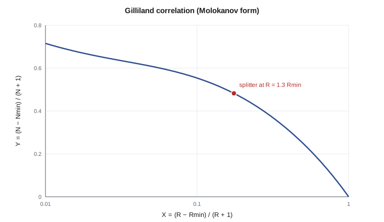
Between the two limits, the Gilliland correlation relates the number of stages at a given reflux to the minimum values through two dimensionless groups, \(X = (R - R_{min})/(R + 1)\) and \(Y = (N - N_{min})/(N + 1)\). Edwin Gilliland plotted it from many stage-by-stage calculations in 1940; the Molokanov equation used here is a common curve fit:
Finally, the Kirkbride equation estimates the optimum feed location as the ratio of stages above and below the feed:
Together the four steps are called the Fenske-Underwood-Gilliland method, often with Kirkbride's feed location added.
# Fenske-Underwood-Gilliland shortcut design of the fusel-alcohol splitter
# Average relative volatilities (to isobutanol) are illustrative values for a dried alcohol cut.
comps = ['ethanol', 'n-propanol', 'isobutanol', 'isoamyl alcohol']
alpha = [2.30, 1.60, 1.00, 0.55]
zF = [0.10, 0.40, 0.30, 0.20]     # mole fractions in a saturated-liquid feed
F = 2.0                            # kmol/h of dried fusel cut pooled from three plants
LK, HK = 1, 2                      # n-propanol light key, isobutanol heavy key
recLK, recHK = 0.98, 0.02          # fractions of LK and HK sent overhead
import math
# Fenske: minimum stages at total reflux
Nmin = math.log((recLK / (1 - recLK)) * ((1 - recHK) / recHK)) / math.log(alpha[LK] / alpha[HK])
print(f"Fenske minimum stages Nmin = {Nmin:.2f}")
# distribute the non-keys with the Fenske equation
d, b = [], []
for a, z in zip(alpha, zF):
    f = F * z
    r = (recHK / (1 - recHK)) * (a / alpha[HK]) ** Nmin   # d_i / b_i
    d.append(f * r / (1 + r)); b.append(f / (1 + r))
D, B = sum(d), sum(b)
for c, di, bi in zip(comps, d, b):
    print(f"{c:16s} distillate {di:7.4f}   bottoms {bi:7.4f} kmol/h")
print(f"D = {D:.3f} kmol/h, B = {B:.3f} kmol/h")
# Underwood: find theta between alpha_HK and alpha_LK with q = 1
q = 1.0
def g(th): return sum(a * z / (a - th) for a, z in zip(alpha, zF)) - (1 - q)
lo, hi = alpha[HK] + 1e-6, alpha[LK] - 1e-6
for _ in range(100):
    m = (lo + hi) / 2
    if g(lo) * g(m) <= 0: hi = m
    else: lo = m
th = (lo + hi) / 2
xD = [di / D for di in d]
Rmin = sum(a * x / (a - th) for a, x in zip(alpha, xD)) - 1
print(f"Underwood theta = {th:.4f}, minimum reflux Rmin = {Rmin:.3f}")
# Gilliland correlation (Molokanov form) at R = 1.3 Rmin
for fac in (1.2, 1.3, 1.5):
    R = fac * Rmin
    X = (R - Rmin) / (R + 1)
    Y = 1 - math.exp((1 + 54.4 * X) / (11 + 117.2 * X) * (X - 1) / math.sqrt(X))
    N = (Y + Nmin) / (1 - Y)
    print(f"R = {fac:.1f} Rmin = {R:.2f}: Gilliland X = {X:.3f}, Y = {Y:.3f}, N = {N:.1f} theoretical stages")
# Kirkbride feed location at R = 1.3 Rmin
R = 1.3 * Rmin; X = (R - Rmin) / (R + 1)
Y = 1 - math.exp((1 + 54.4 * X) / (11 + 117.2 * X) * (X - 1) / math.sqrt(X)); N = (Y + Nmin) / (1 - Y)
xLKB, xHKD = b[LK] / B, d[HK] / D
ratio = ((zF[HK] / zF[LK]) * (xLKB / xHKD) ** 2 * (B / D)) ** 0.206
NR = N * ratio / (1 + ratio)
print(f"Kirkbride: rectifying/stripping = {ratio:.3f}; feed about stage {NR:.1f} from the top of {N:.1f}")Fenske minimum stages Nmin = 16.56 ethanol distillate 0.2000 bottoms 0.0000 kmol/h n-propanol distillate 0.7840 bottoms 0.0160 kmol/h isobutanol distillate 0.0120 bottoms 0.5880 kmol/h isoamyl alcohol distillate 0.0000 bottoms 0.4000 kmol/h D = 0.996 kmol/h, B = 1.004 kmol/h Underwood theta = 1.1886, minimum reflux Rmin = 2.413 R = 1.2 Rmin = 2.90: Gilliland X = 0.124, Y = 0.530, N = 36.4 theoretical stages R = 1.3 Rmin = 3.14: Gilliland X = 0.175, Y = 0.482, N = 32.9 theoretical stages R = 1.5 Rmin = 3.62: Gilliland X = 0.261, Y = 0.410, N = 28.8 theoretical stages Kirkbride: rectifying/stripping = 1.059; feed about stage 16.9 from the top of 32.9
What the numbers say
The keys are close, \(\alpha = 1.6\), and the specification is tight, so the minimum is already 16.6 stages. Ethanol goes overhead completely and isoamyl alcohol to the bottoms completely, as expected for non-keys this far from the keys. The distillate is about 1.0 kmol/h of 79 mol % n-propanol with 20 % ethanol and about 1 % isobutanol, and the bottoms about 1.0 kmol/h of isobutanol and isoamyl alcohol with a little n-propanol.
Underwood's root is \(\theta = 1.189\), between the key volatilities of 1.6 and 1.0, and the minimum reflux is 2.41. At 1.3 times the minimum, \(R = 3.14\), Gilliland gives about 33 equilibrium stages, and Kirkbride puts the feed near the middle, about 17 stages from the top. At 1.2 times the minimum the stages rise to 36; at 1.5 times they fall to 29.
Worked problem
A Fenske check by hand
Verify \(N_{min}\) for 98 % of the light key overhead and 2 % of the heavy key overhead with \(\alpha = 1.6\).
Show solution
- \(d_{LK}/b_{LK} = 0.98/0.02 = 49\); \(b_{HK}/d_{HK} = 0.98/0.02 = 49\).
- Numerator: \(\ln(49 \times 49) = \ln 2401 = 7.784\).
- Denominator: \(\ln 1.6 = 0.470\).
- \(N_{min} = 7.784/0.470 = 16.6\).
Answer: At least 16.6 equilibrium stages, including the reboiler, even at total reflux.
Is the column worth building?
Thirty-three equilibrium stages and a reflux ratio above 3 for a feed of only 150 kg/h is a lot of column for little product. At 60 % efficiency the column would need about 55 trays, or around 20 m of structured packing in a small diameter. Theo works through what would make it cheaper. Relaxing the n-propanol recovery from 98 % to 95 %, while keeping the 2 % isobutanol limit, cuts the minimum stages by about two; relaxing the isobutanol limit cuts them further. Because the key volatility is close to 1, small changes in specification make large changes in size: \(N_{min}\) is inversely proportional to \(\ln\alpha\), which is only 0.47 here.
He also checks the order of separation. The ethanol in the feed ends up in the n-propanol product and lowers its value. A two-column sequence that first removes the ethanol, an easy split with relative volatility 1.44 to n-propanol, could raise the product purity. The heuristics of lesson 1, easy splits first and the most difficult with the fewest other components present, suggest that ordering. Ingrid's reply is practical: the buyer's specification allows ethanol, so one column is enough, and the decision will depend on the price the buyer offers per kilogram of n-propanol against the boiler fuel the fusel oil now replaces.
Reading a shortcut report
When a simulator's shortcut block or a hand calculation returns its numbers, Ingrid's habit is to check four things before anyone uses them. First, the material balance: each component's distillate and bottoms flows must add up to its feed, and the product purities must be possible. Here the distillate carries 0.784 kmol/h of n-propanol out of 0.800 and only 0.012 kmol/h of isobutanol, so the split matches the specification exactly. Second, the non-key distribution: a light non-key that shows up in the bottoms, or a heavy non-key in the distillate, signals either a mistake in the volatilities or keys chosen too far apart. Third, the order of magnitude of \(R_{min}\): for keys this close it should be several times larger than for an easy split, and 2.4 is plausible. Fourth, the ratio \(R/R_{min}\) and \(N/N_{min}\): designs with \(N\) about twice \(N_{min}\) and \(R\) about 1.2 to 1.5 times \(R_{min}\) usually sit near the economic optimum.
Shortcut results also make good sensitivity studies, because they run instantly. Theo tabulates stages and reflux for n-propanol recoveries of 95, 97 and 98 % and isobutanol limits of 1, 2 and 4 %, and gives the table to the commercial team. Seeing that the 1 % limit adds about three equilibrium stages, while 4 % removes about three, lets the buyer and the plant agree a specification on the basis of cost rather than habit. A rigorous simulation then confirms only the chosen case.
Limits of the shortcut methods
The shortcuts assume constant relative volatility and constant molar overflow. They are poor for strongly non-ideal mixtures, mixtures with azeotropes, and columns with large temperature ranges where \(\alpha\) changes. For ethanol-water, they would give nonsense, because \(\alpha\) varies from about 9 to 1 across the column. They are also weak for side draws and multiple feeds. For those cases the next step is a rigorous stage-by-stage calculation, which uses the shortcut results as its starting point.
Common mistakes
MistakePicking keys that are not adjacent in volatility without checking distributed components.
InsteadComponents between the keys distribute; check them with the Fenske equation.
MistakeUsing shortcut methods on a non-ideal or azeotropic mixture.
InsteadThey need roughly constant relative volatility; use rigorous methods otherwise.
MistakeTaking an Underwood root outside the key volatilities.
InsteadThe root used for \(R_{min}\) lies between \(\alpha_{HK}\) and \(\alpha_{LK}\).
MistakeTreating the Gilliland number as real trays.
InsteadIt gives equilibrium stages; divide by an efficiency.
Summary and key terms
- Light and heavy keys define a multicomponent split; non-keys go almost entirely to one product.
- Fenske gives the minimum stages, 16.6 for the fusel splitter.
- Underwood gives the minimum reflux, 2.41.
- Gilliland gives about 33 stages at 1.3 times the minimum; Kirkbride puts the feed near the middle.
- Close keys make the column large; small changes in specification change its size a lot.
- Light key
- The heaviest component that must mostly go to the distillate.
- Heavy key
- The lightest component that must mostly go to the bottoms.
- Non-key
- A component lighter than the light key or heavier than the heavy key.
- Fenske equation
- The minimum number of stages at total reflux for constant relative volatility.
- Underwood equations
- Equations giving the minimum reflux for constant relative volatilities.
- Gilliland correlation
- A correlation relating actual stages and reflux to their minimum values.
Practice problems
Work each problem on paper first, then reveal the answer to check.
With the same keys, what is \(N_{min}\) for 95 % of the light key overhead and 2 % of the heavy key overhead?
Show answer
\(\ln[(0.95/0.05)(0.98/0.02)]/\ln 1.6 = \ln 931/0.470 = 14.5\).
If \(\alpha_{LK,HK}\) were 2.0, what would \(N_{min}\) be for the original specification?
Show answer
\(7.784/\ln 2 = 11.2\).
Between which values does the Underwood root lie here?
Show answer
Between 1.0 and 1.6.
Compute Gilliland \(X\) for \(R = 3.62\) and \(R_{min} = 2.41\).
Show answer
\(1.21/4.62 = 0.26\).
Why is the Kirkbride ratio close to 1 for this column?
Show answer
The feed is split nearly evenly between distillate and bottoms with symmetric key recoveries.
Why can't the shortcuts be used for the wet fusel oil?
Show answer
It forms two liquid phases and is strongly non-ideal.
Lesson quiz · 5 questions
Score 60% or more to complete this lesson.
Create a free account to save your progress, take quizzes and earn a certificate.