
BIOL-499 · Lesson 9 of 12 · 20 min
Data analysis: estimating effects, uncertainty and interpretation
▶ Video coming soon A video version of this lesson is on the way.
Analysis turns data into answers. For an honours project, the goal is not to use the most sophisticated method available but to use a method that matches the design, to estimate the quantities that answer the question, to state the uncertainty in those estimates honestly, and to interpret them without overreaching. This lesson follows Priya's analysis from October to December 2025, using her real, and slightly disappointing, results. All data are invented for this course, but they are typical of what honours projects produce.
Start with a plan and a picture
Priya's proposal had already set out her main analyses: the within-pair ratio of fenced to grazed values for turbidity, calling and tadpole density, each estimated with a 95 in 100 confidence interval and tested with a paired permutation test, plus a regression of tadpole density on turbidity across wetlands. Having that plan meant she did not have to decide, after seeing the data, which comparison to emphasize.
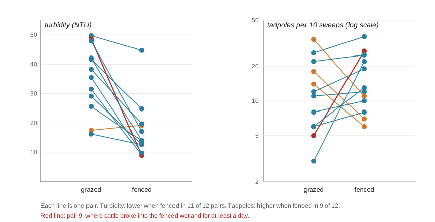
Before running any test, she plotted the data. Plots reveal outliers, errors, skewed distributions and patterns that summary statistics hide. Her first plot showed each pair as two points joined by a line, fenced on one side and grazed on the other. For turbidity, almost every line sloped down toward the fenced side. For tadpoles, most lines sloped up toward the fenced side, but several sloped the other way, and the differences varied enormously in size.
Estimating the effect with a paired analysis
Because each pair shares pasture, soils and weather, the natural measure of the fencing effect is the difference within each pair. Priya worked with ratios on a logarithmic scale, because tadpole counts and turbidity vary multiplicatively: a fence that halves turbidity should look the same in a clear wetland and a muddy one. The mean of the log ratios, converted back to a ratio, is the geometric mean ratio. She used two methods that make few assumptions about the shape of the data: a permutation test, which asks how often randomly flipping which wetland in each pair is called fenced would produce a mean ratio as extreme as the one observed, and a bootstrap, which resamples pairs with replacement to estimate a confidence interval.
# Paired analysis: geometric mean ratio (fenced / grazed), bootstrap CI and exact permutation test.
import numpy as np
from itertools import product
turb_g = np.array([17.5, 38.3, 31.5, 25.6, 16.2, 49.7, 29.1, 41.7, 48.6, 42.1, 35.5, 47.9])
turb_f = np.array([19.2, 19.7, 9.0, 13.9, 12.6, 44.7, 12.7, 24.8, 8.9, 13.9, 9.7, 17.1])
tad_g = np.array([26, 11, 34, 12, 3, 8, 18, 6, 5, 14, 22, 6])     # tadpoles per 10 sweeps
tad_f = np.array([36, 12, 11, 19, 22, 10, 7, 8, 27, 6, 25, 13])
call_g = np.array([14, 9, 17, 10, 6, 8, 12, 7, 5, 11, 15, 6])     # nights with full chorus, of 30
call_f = np.array([18, 10, 9, 13, 16, 9, 7, 8, 17, 6, 16, 11])
rng = np.random.default_rng(2026)
def paired(f, g, name):
    d = np.log(f) - np.log(g)
    signs = np.array(list(product([1, -1], repeat=len(d))))      # all 4,096 sign flips
    p = np.mean(np.abs((signs * d).mean(axis=1)) >= abs(d.mean()) - 1e-12)
    boot = rng.choice(d, (10000, len(d))).mean(axis=1)
    lo, hi = np.exp(np.percentile(boot, [2.5, 97.5]))
    print(f"{name:15s} ratio {np.exp(d.mean()):.2f}  CI {lo:.2f} to {hi:.2f}  p = {p:.3f}")
paired(turb_f, turb_g, "turbidity")
paired(tad_f, tad_g, "tadpoles")
paired(call_f, call_g, "calling nights")turbidity ratio 0.46 CI 0.35 to 0.62 p = 0.001 tadpoles ratio 1.29 CI 0.78 to 2.20 p = 0.380 calling nights ratio 1.18 CI 0.86 to 1.61 p = 0.354
The results answered Priya's three predictions in three different ways. Turbidity in fenced wetlands was about 0.46 times that in grazed wetlands, less than half, with a confidence interval of about 0.35 to 0.62 and a permutation p-value of about 0.001. Fencing very likely reduces turbidity, and the effect is large. Tadpole densities were about 1.29 times higher in fenced wetlands, with a confidence interval from about 0.78 to 2.20 and a p-value of about 0.38. Calling nights were about 1.18 times higher, with an interval from about 0.86 to 1.61. Neither biological response showed a statistically clear difference.
Interpreting confidence intervals and p-values
A p-value is the probability of obtaining a result at least as extreme as the one observed if the null hypothesis, here no effect of fencing, were true. A small p-value says the data would be surprising if there were no effect; it does not give the probability that the hypothesis is true, and it does not say how large or important the effect is. A p-value of 0.38 does not show that fencing has no effect on tadpoles. It shows only that these data are quite compatible with no effect.
A confidence interval is more informative because it shows the range of effect sizes compatible with the data. Priya's interval for tadpoles, 0.78 to 2.20, says that the data are compatible with fencing reducing tadpole density by about a fifth, increasing it more than twofold, or anything in between. They are not compatible with very large effects in either direction: a fourfold increase, for example, is outside the interval. That is real information. Combined with the power analysis from lesson 5, which showed only about a 7 in 10 chance of detecting a 1.6-fold effect with 12 pairs, it suggests that the study was too small to settle the question rather than that fencing does nothing.
Many statisticians now recommend reporting effect sizes and confidence intervals as the main results and treating p-values as secondary, avoiding language such as significant and not significant as if they divided effects into real and absent. Priya's thesis reported every estimate with its interval, described the turbidity result as strong evidence of a large reduction, and described the tadpole and calling results as estimates favouring fenced wetlands but too uncertain to exclude no effect or a modest negative effect.
| Response | Ratio, fenced to grazed | 95 in 100 interval | Interpretation |
|---|---|---|---|
| Turbidity | 0.46 | 0.35 to 0.62 | Large, clear reduction with fencing |
| Tadpole density | 1.29 | 0.78 to 2.20 | Favours fenced wetlands, but compatible with no effect or a small decrease |
| Calling nights | 1.18 | 0.86 to 1.61 | Similar pattern, also uncertain |
Testing the mechanism
Priya's hypothesis said fencing would help frogs through lower turbidity. If so, wetlands with lower turbidity should have more tadpoles. She examined this in two ways: across all 24 wetlands, and within pairs, asking whether pairs with larger turbidity reductions had larger tadpole gains.
# Is tadpole density related to turbidity? Across all wetlands and within pairs.
import numpy as np
from scipy import stats
turb_g = np.array([17.5, 38.3, 31.5, 25.6, 16.2, 49.7, 29.1, 41.7, 48.6, 42.1, 35.5, 47.9])
turb_f = np.array([19.2, 19.7, 9.0, 13.9, 12.6, 44.7, 12.7, 24.8, 8.9, 13.9, 9.7, 17.1])
tad_g = np.array([26, 11, 34, 12, 3, 8, 18, 6, 5, 14, 22, 6])
tad_f = np.array([36, 12, 11, 19, 22, 10, 7, 8, 27, 6, 25, 13])
across = stats.linregress(np.r_[turb_g, turb_f], np.log(np.r_[tad_g, tad_f]))
print(f"across 24 wetlands: slope {across.slope:.4f} per NTU, r = {across.rvalue:.2f}, p = {across.pvalue:.2f}")
print(f"  a 10 NTU increase multiplies density by about {np.exp(10 * across.slope):.2f}")
within = stats.linregress(turb_f - turb_g, np.log(tad_f) - np.log(tad_g))
print(f"within 12 pairs: slope {within.slope:.4f} per NTU, r = {within.rvalue:.2f}, p = {within.pvalue:.2f}")across 24 wetlands: slope -0.0151 per NTU, r = -0.32, p = 0.13 a 10 NTU increase multiplies density by about 0.86 within 12 pairs: slope 0.0038 per NTU, r = 0.05, p = 0.88
Across all wetlands, tadpole density tended to be lower where water was more turbid: each additional 10 NTU was associated with about 14 in 100 fewer tadpoles, but the relationship was weak, with a correlation of about minus 0.32 and a p-value of about 0.13. Within pairs, there was no relationship at all: pairs where fencing reduced turbidity the most did not show the largest tadpole gains. The mechanism prediction was therefore not supported by these data. Turbidity may matter less to chorus frog tadpoles than expected, or its effects may be masked by other differences among wetlands, such as predators, depth or how long the wetland held water.
Priya was careful not to over-interpret a correlation across wetlands. Wetlands differ in many ways, and a correlation between turbidity and tadpoles across wetlands could arise because both are linked to something else, such as wetland depth. The within-pair analysis controls for many of those differences and is the stronger test.
Sensitivity analysis
A sensitivity analysis asks whether a conclusion changes when a reasonable alternative choice is made. Priya's field notebook recorded that cattle had broken into fenced wetland F9 for at least a day in early June. Pair 9 also had one of the largest tadpole differences in favour of fencing. She reran the tadpole analysis without pair 9. The ratio fell from about 1.29 to about 1.13, with an interval of about 0.70 to 1.88, and the conclusion, an uncertain estimate favouring fenced wetlands, did not change. She reported both versions. Reporting a sensitivity analysis shows readers how much the result depends on particular decisions, and it is far more convincing than quietly choosing whichever version looks better.
The eDNA results
For her third aim, Priya compared eDNA detection with calling records, which showed frogs breeding at all 24 wetlands. Before dilution, chorus frog DNA was detected in most qPCR replicates from fenced wetlands but in far fewer from grazed wetlands, and one grazed wetland had no detections at all despite calling on 8 nights. After diluting inhibited extracts, detection rose in grazed wetlands to rates similar to fenced ones. Her conclusion was methodological: in turbid prairie wetlands, inhibition can create false absences and false differences between treatments, so eDNA surveys must include an internal positive control and dilute inhibited samples. This was the most novel finding of her project, and it came from following up a result that did not make sense.
Planned and exploratory analyses
After seeing the data, Priya noticed that tadpoles seemed more abundant in deeper wetlands, whatever the treatment. She explored this with a plot and a simple regression and found a positive association. Because she had not planned this analysis, she labelled it exploratory in her thesis and suggested it as a question for future work, rather than presenting it as a finding. The distinction matters. If enough unplanned comparisons are run, some will produce small p-values by chance alone: with 20 independent tests of true null hypotheses at a threshold of 0.05, about one is expected to be significant. Reporting how many analyses were run, and which were planned, lets readers judge the evidence.
Choosing methods and checking assumptions
Priya's permutation tests and bootstrap intervals were well suited to 12 pairs with skewed data, because they make few assumptions. A paired t-test on the log ratios gave very similar results, which she reported in an appendix. More complex methods, such as generalized linear mixed models with wetland and visit as random effects and counts per sweep as the response, would use all the subsample information and are common in ecological papers. Dr. Szabo helped her fit one as a check, and it gave a similar estimate with a similar interval. For an honours thesis, a simple, correct analysis that you understand well and can explain in a defence is better than a complex one you cannot.
Whatever method is used, its assumptions should be checked. For regression, plot the residuals against fitted values to look for curvature or uneven spread; for tests based on the normal distribution, check that the differences are not strongly skewed; for any analysis, check that the units of analysis are independent. Report what you checked.
Worked problem
Reading a confidence interval
A study of fencing and wood frog tadpoles in another region reports a ratio of 1.05 with a 95 in 100 confidence interval of 0.95 to 1.16, from 40 pairs. Compare its information with Priya's tadpole result, a ratio of 1.29 with an interval of 0.78 to 2.20 from 12 pairs.
Show solution
- Both intervals include 1, so neither study gives clear evidence of an effect.
- The other study's interval is narrow: it rules out effects larger than about a 16 in 100 increase or a 5 in 100 decrease.
- Priya's interval is wide: it is compatible with anything from about a 22 in 100 decrease to a 120 in 100 increase.
- So the other study is informative about the absence of large effects, while Priya's study is mostly informative that very large effects are unlikely.
Answer: Neither result is significant, but they say very different things. The 40-pair study shows that any effect is small; Priya's 12-pair study leaves a wide range of effects possible. Precision, shown by interval width, matters as much as whether an interval includes 1.
Common mistakes
MistakeA p-value of 0.38 shows that fencing has no effect.
InsteadIt shows the data are compatible with no effect; the confidence interval shows which effect sizes remain plausible.
MistakeA small p-value means a large or important effect.
InsteadSmall p-values can come from tiny effects with large samples; report effect sizes and intervals.
MistakeExploratory findings should be presented as results.
InsteadLabel unplanned analyses as exploratory and report how many were run.
MistakeRemoving an awkward data point is acceptable if it improves the result.
InsteadExclude data only for documented reasons, and report results with and without the exclusion.
Summary and key terms
- Plan analyses in advance, plot the data first and match the analysis to the design and its experimental units.
- Paired designs are analysed with within-pair differences or ratios; log ratios suit multiplicative effects.
- Permutation tests and bootstrap intervals make few assumptions and suit small samples.
- Confidence intervals show which effect sizes are compatible with the data; p-values alone do not show size or importance.
- Test mechanisms with appropriate comparisons, prefer within-pair tests to cross-site correlations, and report sensitivity analyses.
- Separate planned from exploratory analyses, check assumptions and prefer methods you can explain.
- Effect size
- A measure of the magnitude of a difference or relationship, such as a ratio or a mean difference.
- Confidence interval
- A range of values compatible with the data at a chosen confidence level, showing the precision of an estimate.
- p-value
- The probability of a result at least as extreme as observed if the null hypothesis were true.
- Permutation test
- A test that compares the observed statistic with its distribution under random rearrangements of the data.
- Bootstrap
- A method that estimates uncertainty by repeatedly resampling the data with replacement.
- Sensitivity analysis
- Repeating an analysis with alternative reasonable choices to see whether conclusions change.
Practice problems
Work each problem on paper first, then reveal the answer to check.
The log ratio of fenced to grazed turbidity averages minus 0.78. What is the geometric mean ratio?
Show answer
e to the power minus 0.78 is about 0.46, so fenced wetlands have about 0.46 times the turbidity.
An interval for a ratio is 0.78 to 2.20. Is a ratio of 1 compatible with the data? Is 3?
Show answer
1 is inside the interval, so it is compatible; 3 is outside, so it is not.
Why is the within-pair regression a stronger test of the turbidity mechanism than the regression across all wetlands?
Show answer
Pairs share many characteristics, so within-pair comparisons control for differences among wetlands that could confound a cross-site correlation.
With 20 independent tests of true null hypotheses at a 0.05 threshold, how many significant results are expected by chance?
Show answer
20 times 0.05, which is 1.
Lesson quiz · 5 questions
Score 60% or more to complete this lesson.
Create a free account to save your progress, take quizzes and earn a certificate.