
BIOL-499 · Lesson 7 of 12 · 20 min
In the field and the lab: protocols, notebooks and quality control
▶ Video coming soon A video version of this lesson is on the way.
Collecting data is where a research plan meets reality. Recorders fail, nets tear, a thunderstorm ends a sampling day, and a reagent behaves differently from the last batch. The quality of a data set depends less on any single measurement than on the systems that surround measurement: written protocols that everyone follows, records that capture what actually happened, checks that catch errors early, and controls that reveal problems hidden in the data. This lesson follows Priya through her field season from late April to July 2025 and her eDNA lab work in the fall, and it describes the most important discovery of her project, which came from a quality control check.
Protocols
A protocol, or standard operating procedure, is a written, step-by-step description of how a task is done. It ensures that a measurement means the same thing every time, whoever makes it, and it allows someone else to repeat the work. Priya wrote or adapted a protocol for every procedure: deploying and checking recorders, measuring turbidity, dip-netting, collecting and filtering eDNA samples, decontaminating gear and scoring recordings. Each protocol had a version number and date, and when she changed one, she updated the version and recorded the change in her project log.
A good protocol is specific. Measure turbidity is not a protocol. Rinse the sample cell three times with wetland water; fill to the line from 10 centimetres below the surface, 1 metre from the margin; wipe the cell with lint-free tissue; take three readings and record all three; recalibrate with the standards at the start of each field day is a protocol. The specificity matters because small differences, such as sampling near the bottom where sediment is stirred up, can produce differences larger than the effect being studied.
Before the season, Priya tested her protocols in a pilot: two days at four wetlands not in the study. The pilot showed that her original plan of five dip-net sweeps per visit gave very variable counts, so she increased to ten, and that filtering a full litre of water through the eDNA filter took over twenty minutes in the most turbid wetlands, so she brought a second hand pump. Pilots are the cheapest way to find problems.
Field and lab notebooks
The research notebook is the primary record of what was done, when, by whom and with what result. It is also a legal and ethical record: in cases of disputed results or inventions, notebooks are evidence. Traditional notebooks are bound, with numbered pages, entries in ink, dated and never removed; errors are struck through with a single line so they remain readable. Electronic lab notebooks provide the same features digitally, with time stamps and audit trails, and many universities now provide them.
In the field, Priya used printed data sheets on waterproof paper, one per wetland visit, with spaces for every variable in the protocol, plus a bound field notebook for observations that did not fit the sheet: a broken fence, an unusual weather event, cattle seen inside a fenced wetland, or a note that the turbidimeter's battery was low. Each evening she photographed the day's sheets, so that a lost clipboard would not lose data, and entered the data into a spreadsheet within 48 hours, while her memory could still resolve unclear handwriting.
| Good practice | Why |
|---|---|
| Record data directly on the sheet, never on scraps to copy later | Copying introduces errors and loses the original |
| Record units and the instrument used | A value without units or method is ambiguous |
| Record zero as 0 and missing as a clear code | Blank cells are ambiguous: was it zero, missing or forgotten? |
| Note anything unusual, even if it seems unimportant | Unusual events often explain outliers later |
| Strike through errors with one line and initial them | Keeps the original record visible |
| Photograph or scan sheets daily | Protects against loss and damage |
One entry in Priya's field notebook later proved important: on 3 June, she noted that cattle had broken into fenced wetland F9 for at least a day before the rancher repaired the fence. Because she recorded it, she could check whether excluding that pair changed her results, and report the incident honestly in her thesis.
Calibration and measurement error
Instruments drift. Priya's turbidimeter was calibrated at the start of each field day against commercial standards of known turbidity, and she recorded each calibration in the notebook. Once a week she also measured a check standard, a sample of known value not used for calibration, to confirm the meter was reading correctly. Her automated recorders were set to the same gain and sampling rate, and each was tested with a standard tone before deployment.
Measurement error has two parts. Random error makes repeated measurements scatter around the true value and is reduced by averaging, which is why Priya took three turbidity readings and averaged them. Systematic error, or bias, shifts all measurements in one direction and is not reduced by averaging; it is caught by calibration, check standards and comparing methods. A meter that reads 2 NTU too high every time gives precise but inaccurate data.
eDNA in the field: avoiding contamination
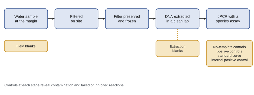
Environmental DNA methods are extraordinarily sensitive, which is their strength and their main weakness. A few copies of DNA carried on a glove or a net from a wetland with frogs to one without can produce a false positive. eDNA sampling therefore follows strict contamination controls.
- Clean equipment: Priya used new single-use filter housings and gloves for each wetland and decontaminated reusable equipment with dilute bleach, which destroys DNA, followed by rinsing.
- Order of sampling: water samples were collected before anyone entered the water for dip-netting, so that disturbance did not stir up sediment or transfer DNA.
- Field blanks: at each of eight wetlands, she filtered one litre of purified water brought from the lab, handled exactly like a real sample. Any frog DNA in a blank would indicate contamination during sampling.
- Preservation: filters were placed in tubes with preservative and kept cool, then frozen at the station within hours.
eDNA in the lab: controls and the qPCR standard curve
Back at the university in September, Priya extracted DNA from her 72 filters and 8 field blanks in a dedicated clean room, separated from the rooms where DNA is amplified, because amplified DNA is the most common source of lab contamination. Extraction blanks, tubes with no filter taken through every step, tested for contamination during extraction. The chorus frog assay was quantitative PCR, or qPCR, which detects a short species-specific sequence of mitochondrial DNA and measures how many cycles of amplification are needed before the fluorescent signal crosses a threshold. That number is the quantification cycle, or Cq, also called the Ct. Fewer cycles mean more starting DNA.
Every qPCR plate included no-template controls, wells with water instead of DNA, which must stay negative; positive controls of known chorus frog DNA, which must amplify; and a dilution series of a synthetic DNA standard of known copy number, which gives the standard curve. The slope of Cq against the logarithm of copy number shows how efficiently the reaction doubles the DNA each cycle.
# qPCR standard curve: Cq for a tenfold dilution series of a synthetic standard.
import numpy as np
log_copies = np.array([1, 2, 3, 4, 5])           # 10 to 100,000 copies per reaction
cq = np.array([34.1, 30.8, 27.4, 24.0, 20.7])
slope, intercept = np.polyfit(log_copies, cq, 1)
efficiency = 10 ** (-1 / slope) - 1
r2 = np.corrcoef(log_copies, cq)[0, 1] ** 2
print(f"slope = {slope:.2f}, intercept = {intercept:.2f}")
print(f"efficiency = {efficiency:.3f} (1.00 means perfect doubling each cycle)")
print(f"R squared = {r2:.4f}")
sample_cq = 31.9
print(f"a sample with Cq {sample_cq} has about {10 ** ((sample_cq - intercept) / slope):.0f} copies")slope = -3.36, intercept = 37.48 efficiency = 0.984 (1.00 means perfect doubling each cycle) R squared = 1.0000 a sample with Cq 31.9 has about 46 copies
A perfectly efficient reaction doubles the DNA each cycle, so a tenfold dilution should add log base 2 of 10, about 3.32 cycles: a slope of about minus 3.32. Priya's slope of minus 3.36 gave an efficiency of about 0.98, within the range of 0.90 to 1.10 usually accepted, and the standard points fell almost exactly on a line. All no-template controls, extraction blanks and field blanks were negative, so there was no evidence of contamination.
The discovery: inhibition
When Priya compared her first eDNA results with the recorder data, something was wrong. Every one of her 24 wetlands had chorus frog calling recorded on at least several nights, so frogs were certainly breeding in all of them. Yet several grazed wetlands had chorus frog DNA in only one or two of their nine qPCR replicates, and one had none at all. The fenced wetlands, by contrast, were positive in most replicates. A naive reading would be that grazed wetlands had far fewer frogs. But Mei Chen suggested checking the internal positive control.
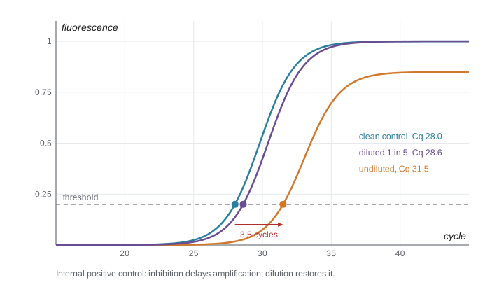
An internal positive control, or IPC, is a synthetic DNA sequence added in a known amount to every reaction and detected with its own fluorescent probe. If nothing interferes, the IPC amplifies at the same Cq in every well. If the sample contains substances that inhibit the polymerase, such as humic acids and fine sediment common in turbid water, the IPC is delayed. A delay of more than about 1.5 cycles compared with the no-template controls was Priya's lab's threshold for flagging inhibition.
# IPC delay (cycles later than in clean controls) and turbidity for each wetland pair.
import numpy as np
turb_grazed = np.array([17.5, 38.3, 31.5, 25.6, 16.2, 49.7, 29.1, 41.7, 48.6, 42.1, 35.5, 47.9])
turb_fenced = np.array([19.2, 19.7, 9.0, 13.9, 12.6, 44.7, 12.7, 24.8, 8.9, 13.9, 9.7, 17.1])
ipc_grazed = np.array([1.6, 2.2, 2.6, 1.3, 1.1, 3.6, 2.3, 3.5, 3.1, 3.4, 1.9, 3.9])
ipc_fenced = np.array([0.8, 1.4, 0.5, 0.4, 0.9, 3.0, 0.3, 1.9, 0.6, 0.5, 0.7, 1.2])
print("inhibited (delay > 1.5 cycles): grazed", int((ipc_grazed > 1.5).sum()), "of 12;",
      "fenced", int((ipc_fenced > 1.5).sum()), "of 12")
turb = np.concatenate([turb_grazed, turb_fenced]); ipc = np.concatenate([ipc_grazed, ipc_fenced])
print(f"correlation of IPC delay with turbidity: r = {np.corrcoef(turb, ipc)[0, 1]:.2f}")inhibited (delay > 1.5 cycles): grazed 10 of 12; fenced 2 of 12 correlation of IPC delay with turbidity: r = 0.95
Ten of the twelve grazed wetlands but only two fenced wetlands showed inhibition, and the IPC delay was strongly correlated with turbidity. The low detection rates in grazed wetlands were not evidence of fewer frogs. They were largely a technical artefact: something in the turbid water was blocking the reaction. Because inhibition was linked to the treatment, it would have biased the comparison of fenced and grazed wetlands if Priya had not caught it.
The standard remedy is to dilute the extract, which dilutes the inhibitors more than it reduces detectability when DNA is plentiful. Priya reran all inhibited extracts at a one-in-five dilution, as her risk plan had allowed, and the IPC delays fell below the threshold in all but one sample. Detection rates in grazed wetlands rose sharply, and the difference between treatments in eDNA detection mostly disappeared. She recorded the decision, the date and the reason in her project log, reported both the undiluted and diluted results in her thesis, and made inhibition one of the main findings of her third aim: in turbid prairie wetlands, eDNA surveys that do not test for inhibition can badly underestimate where a species occurs.
Quality control of data
Quality control continues after collection. Priya used a set of checks on every data file: ranges (turbidity cannot be negative, calling index must be 0 to 3), consistency (every wetland has the expected number of visits), duplicates, and cross-checks between variables (a wetland recorded as dry cannot have tadpole counts). She also double-entered a random tenth of the field sheets and compared the two versions, finding an error rate of about 1 in 400 values, which she then corrected. Lesson 8 describes how she scripted these checks so they could be rerun whenever data changed.
Worked problem
Checking a qPCR plate
A plate has these results: no-template controls negative; positive controls Cq 26.1 and 26.3; standard curve slope minus 4.10; IPC delays under 0.5 cycles for all samples. Should the plate be accepted?
Show solution
- No-template controls are negative, so there is no evidence of contamination.
- Positive controls amplify, so the reaction worked.
- Calculate efficiency: 10 to the power of minus 1 divided by minus 4.10 is 10 to the power 0.244, about 1.75, minus 1 gives 0.75.
- An efficiency of about 0.75 is well below the usual acceptable range of 0.90 to 1.10, suggesting a problem with the standards, reagents or cycling.
Answer: The plate should not be accepted for quantification: the standard curve efficiency is about 0.75. Presence or absence calls might still be usable, but the plate should be rerun with fresh standards before copy numbers are reported.
Common mistakes
MistakeDetection rates from eDNA directly measure how many animals are present.
InsteadDetection depends on DNA amount, sampling, degradation and inhibition; check controls and inhibition before interpreting.
MistakeAveraging repeated readings removes all measurement error.
InsteadAveraging reduces random error but not systematic bias, which needs calibration and check standards.
MistakeNotes about unusual events are unnecessary if the data sheet is complete.
InsteadUnusual events, such as a broken fence, often explain outliers and must be reported.
MistakeNegative controls are only needed if contamination is suspected.
InsteadControls are included every time, because contamination is otherwise invisible.
Summary and key terms
- Written, versioned protocols make measurements consistent and repeatable; pilots reveal problems cheaply.
- Notebooks and data sheets are the primary record: date everything, record units, distinguish zero from missing and note unusual events.
- Calibration and check standards catch systematic error; averaging reduces random error.
- eDNA work needs strict contamination controls: clean equipment, sampling order, field blanks, extraction blanks and no-template controls.
- qPCR standard curves give reaction efficiency; internal positive controls reveal inhibition.
- Priya's inhibition finding showed how a technical artefact linked to the treatment could have biased the results.
- Protocol
- A written step-by-step procedure for carrying out a task in a standard way.
- Field blank
- A sample of clean water handled like a real sample to detect contamination during collection.
- Quantification cycle (Cq)
- The qPCR cycle at which fluorescence crosses a threshold; lower values mean more starting DNA.
- Amplification efficiency
- The proportion by which target DNA increases each PCR cycle; 1.0 means perfect doubling.
- Internal positive control (IPC)
- A known DNA sequence added to each qPCR reaction to detect inhibition.
- PCR inhibition
- Interference with amplification by substances in a sample, such as humic acids or fine sediment.
Practice problems
Work each problem on paper first, then reveal the answer to check.
A standard curve has a slope of minus 3.32. What is the efficiency?
Show answer
10 to the power of 1 divided by 3.32 is about 2.00; minus 1 gives an efficiency of about 1.00, or perfect doubling.
Why were water samples collected before dip-netting?
Show answer
So that disturbance from wading did not stir up sediment or transfer DNA into the samples.
What does a positive field blank indicate?
Show answer
Contamination during sampling or handling, so results from that day must be treated with caution.
Why was inhibition a particular problem for Priya's comparison?
Show answer
It was more common in turbid grazed wetlands, so it was linked to the treatment and would have biased the comparison.
Lesson quiz · 5 questions
Score 60% or more to complete this lesson.
Create a free account to save your progress, take quizzes and earn a certificate.